Lattes, Occhialini, and Powell: the pion’s two-body decay

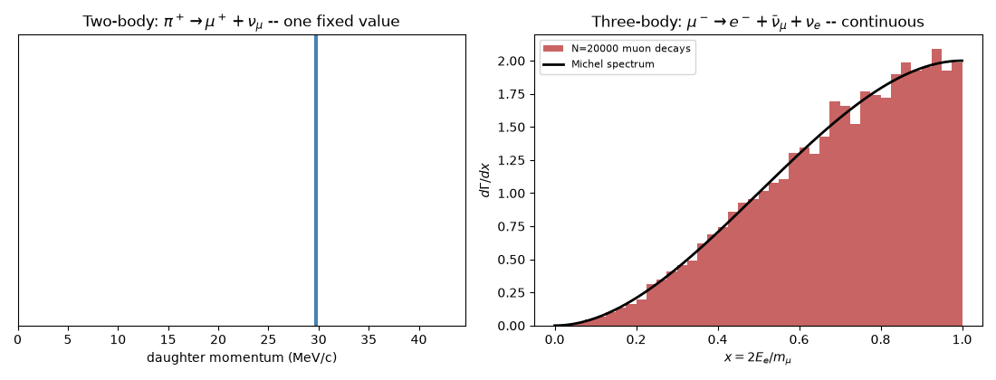
In 1947 Lattes, Occhialini and Powell exposed nuclear emulsion plates on mountaintops and found tracks of a new particle, the charged pion, stopping and decaying into a muon. Every one of those muons had the same track length in the emulsion, about 600 µm. That is the signature of a two-body decay, \(\pi^+\to\mu^++\nu_\mu\): in the pion’s rest frame the muon gets one fixed momentum, however many times the decay is repeated. The muon in turn decayed to an electron with a continuous range of energies, the three-body signature of \(\mu^+\to e^++\nu_e+\bar\nu_\mu\). The whole \(\pi\to\mu\to e\) chain was visible in a single photograph.

This example computes the pion’s fixed daughter momentum with two_body_decay_momentum() and builds the muon’s continuous electron spectrum event by event with muon_decay_event().

import matplotlib.pyplot as plt
import numpy as np

from physicskit.particle.decays import (
    michel_spectrum,
    muon_decay_event,
    sample_michel_electron_energies,
    two_body_decay_momentum,
)
from physicskit.particle.kinematics import invariant_mass
from physicskit.particle.visualizers import animate_michel_histogram

Two-body: the pion’s fixed daughter momentum

pi+ -> mu+ + nu_mu is genuinely two-body: the muon’s momentum in the pion rest frame has one single, sharply fixed value, no matter how many times the decay is repeated.

m_pi, m_mu, m_nu = 139.570, 105.658, 0.0
p_star = two_body_decay_momentum(m_pi, m_mu, m_nu)
print("pi+ -> mu+ + nu_mu (genuinely two-body):")
print(f"  fixed daughter momentum p* = {p_star:.4f} MeV/c, every single time")

pi+ -> mu+ + nu_mu (genuinely two-body):
  fixed daughter momentum p* = 29.7921 MeV/c, every single time

Three-body: the muon’s own continuous spectrum

The muon itself decays three-body, mu- -> e- + nu_mu_bar + nu_e. muon_decay_event() builds one complete event via two chained exact two-body decays; repeated many times, the electron’s energy comes out with a genuinely continuous spread – exactly the signature that, applied to the neutron’s beta decay eight decades earlier, was the puzzle Pauli’s neutrino was invented to resolve.

rng = np.random.default_rng(0)
n_events = 20000
electron_energies = np.empty(n_events)
for i in range(n_events):
    p_e, p_numu_bar, p_nue = muon_decay_event(m_mu, rng=rng)
    electron_energies[i] = p_e.E

x_samples = 2.0 * electron_energies / m_mu  # scaled energy, matching the Michel-spectrum convention
print("\nmu- -> e- + nu_mu_bar + nu_e (genuinely three-body):")
print(f"  electron energy: min={electron_energies.min():.2f}, max={electron_energies.max():.2f} MeV -- a continuous spread, not one fixed value")
print(f"  mean scaled energy <x>: {x_samples.mean():.4f} (theoretical value from the Michel spectrum: 0.7)")

# Cross-check one event's full four-momentum conservation.
rng_check = np.random.default_rng(1)
p_e, p_numu_bar, p_nue = muon_decay_event(m_mu, rng=rng_check)
print(f"  one event's reconstructed invariant mass: {invariant_mass([p_e, p_numu_bar, p_nue]):.6f} MeV (should equal m_mu={m_mu})")

mu- -> e- + nu_mu_bar + nu_e (genuinely three-body):
  electron energy: min=1.82, max=52.83 MeV -- a continuous spread, not one fixed value
  mean scaled energy <x>: 0.7010 (theoretical value from the Michel spectrum: 0.7)
  one event's reconstructed invariant mass: 105.658000 MeV (should equal m_mu=105.658)

Side by side

fig, (ax1, ax2) = plt.subplots(1, 2, figsize=(11, 4.2))
ax1.axvline(p_star, color="steelblue", lw=3)
ax1.set_xlim(0, p_star * 1.5)
ax1.set_yticks([])
ax1.set_xlabel("daughter momentum (MeV/c)")
ax1.set_title(r"Two-body: $\pi^+\to\mu^++\nu_\mu$ -- one fixed value")

x_theory = np.linspace(0, 1, 200)
ax2.hist(x_samples, bins=40, range=(0, 1), density=True, color="firebrick", alpha=0.7, label=f"N={n_events} muon decays")
ax2.plot(x_theory, michel_spectrum(x_theory), color="black", lw=2, label="Michel spectrum")
ax2.set_xlabel(r"$x=2E_e/m_\mu$")
ax2.set_ylabel(r"$d\Gamma/dx$")
ax2.set_title(r"Three-body: $\mu^-\to e^-+\bar\nu_\mu+\nu_e$ -- continuous")
ax2.legend(fontsize=8)
fig.tight_layout()

Building up the spectrum event by event

x_samples_anim = sample_michel_electron_energies(2000, rng=np.random.default_rng(2))
anim = animate_michel_histogram(x_samples_anim, batch_size=40)

plt.show()

Check

Two-body: p* = (m_pi^2 - m_mu^2) / 2 m_pi exactly. Three-body: a continuous Michel spectrum with <x> = 0.7, and four-momentum conserved.

assert abs(p_star - (m_pi**2 - m_mu**2) / (2 * m_pi)) < 1e-9
assert abs(x_samples.mean() - 0.7) < 0.005
assert abs(invariant_mass([p_e, p_numu_bar, p_nue]) - m_mu) < 1e-9