Pontecorvo, Maki, Nakagawa, and Sakata: neutrino oscillations

If neutrinos carry a small mass, nothing forbids oscillation between flavors over macroscopic distances. In the simplest two-flavor treatment, a neutrino produced in flavor \(e\) oscillates into flavor \(\mu\) with probability

\[P(\nu_e\to\nu_\mu) = \sin^2(2\theta)\, \sin^2\!\left(1.267\,\frac{\Delta m^2 L}{E}\right),\]

vanishing identically unless neutrinos have nonzero, non-degenerate masses. This example plots oscillation_probability() and survival_probability() against baseline for parameters close to the atmospheric-oscillation values Super-Kamiokande measured, and shows how the oscillation wavelength and depth depend on the mixing angle and mass-squared splitting separately.

import matplotlib.pyplot as plt
import numpy as np

from physicskit.particle.neutrinos import oscillation_probability, survival_probability
from physicskit.particle.visualizers import animate_neutrino_oscillation

Oscillation vs. baseline, near-atmospheric parameters

theta = np.radians(45.0)  # close to maximal mixing
delta_m2 = 2.5e-3  # eV^2, close to the atmospheric splitting
E = 1.0  # GeV

L = np.linspace(0.0, 2000.0, 1000)  # km
P_mu = oscillation_probability(L, E, theta, delta_m2)
P_e = survival_probability(L, E, theta, delta_m2)

fig1, ax1 = plt.subplots(figsize=(7, 4.5))
ax1.plot(L, P_e, color="steelblue", label=r"$P(\nu_e\to\nu_e)$")
ax1.plot(L, P_mu, color="firebrick", label=r"$P(\nu_e\to\nu_\mu)$")
ax1.set_xlabel("baseline L (km)")
ax1.set_ylabel("probability")
ax1.set_title(f"Two-flavor oscillation (theta=45 deg, dm^2={delta_m2} eV^2, E={E} GeV)")
ax1.legend()
fig1.tight_layout()

print(f"P(nu_e -> nu_e) + P(nu_e -> nu_mu) at every L: {np.allclose(P_e + P_mu, 1.0)}")
print(f"P(nu_mu) at L=0: {P_mu[0]:.6f} (must vanish -- no oscillation with zero baseline)")

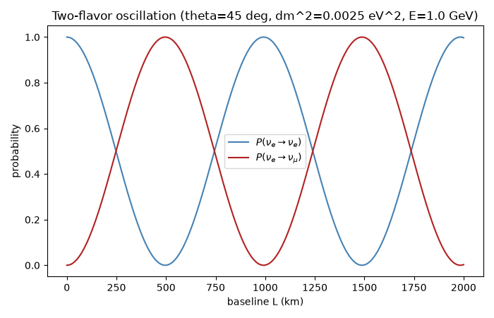
P(nu_e -> nu_e) + P(nu_e -> nu_mu) at every L: True
P(nu_mu) at L=0: 0.000000 (must vanish -- no oscillation with zero baseline)

Mixing angle sets the depth; mass splitting sets the wavelength

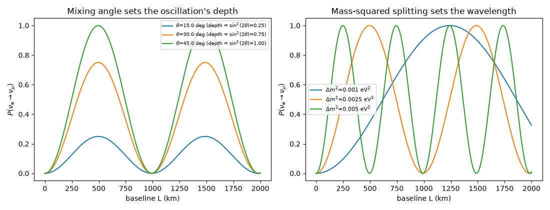
theta alone controls the amplitude sin^2(2theta) (maximal at theta=45 deg); delta_m2 alone controls how quickly the oscillation completes as a function of L/E, independent of theta.

fig2, (ax2, ax3) = plt.subplots(1, 2, figsize=(11, 4.2))
for theta_deg in [15.0, 30.0, 45.0]:
    P = oscillation_probability(L, E, np.radians(theta_deg), delta_m2)
    ax2.plot(L, P, label=rf"$\theta$={theta_deg} deg (depth = $\sin^2(2\theta)$={np.sin(np.radians(2 * theta_deg)) ** 2:.2f})")
ax2.set_xlabel("baseline L (km)")
ax2.set_ylabel(r"$P(\nu_e\to\nu_\mu)$")
ax2.set_title("Mixing angle sets the oscillation's depth")
ax2.legend(fontsize=7)

for dm2 in [1.0e-3, 2.5e-3, 5.0e-3]:
    P = oscillation_probability(L, E, theta, dm2)
    ax3.plot(L, P, label=rf"$\Delta m^2$={dm2} eV$^2$")
ax3.set_xlabel("baseline L (km)")
ax3.set_ylabel(r"$P(\nu_e\to\nu_\mu)$")
ax3.set_title("Mass-squared splitting sets the wavelength")
ax3.legend(fontsize=8)
fig2.tight_layout()

Building up the picture as a function of baseline

anim = animate_neutrino_oscillation(L, E, theta, delta_m2)

plt.show()