Fermi’s theory of beta decay: spectrum shape, Kurie plot, and Sargent’s rule

Fermi (1933-1934) wrote beta decay as a contact interaction of four fermions – neutron, proton, electron, neutrino – at a single point, with one new coupling \(G_F\). For an allowed transition the matrix element is constant, so the electron spectrum is phase space times a Coulomb correction, the Fermi function \(F(Z,E)\):

\[\frac{dN}{dT} \propto F(Z,E)\,pE\,(Q-T)^2 ,\]

with electron momentum \(p\), total energy \(E=T+m_e\) and kinetic energy \(T\). Two consequences made the theory testable. The Kurie plot \(\sqrt{N/(pEF)}\) against \(T\) is a straight line hitting zero exactly at the endpoint \(Q\). The total rate integrates to \(\Gamma\propto G_F^2 Q^5\) for \(Q\gg m_e\), explaining Sargent’s empirical rule that decay rates climb steeply with energy release. This example takes the free neutron’s endpoint from q_value(), then checks both predictions on the tritium spectrum (\(Q=18.6\) keV).

import matplotlib.pyplot as plt
import numpy as np
from scipy.integrate import trapezoid

from physicskit.particle.nuclear import q_value

m_e = 0.51099895  # MeV
alpha = 1 / 137.035999


def fermi_function(Z, T):
    """Non-relativistic Fermi function for an emitted electron, daughter charge Z."""
    E = T + m_e
    p = np.sqrt(E**2 - m_e**2)
    eta = alpha * Z * E / p
    return 2 * np.pi * eta / (1 - np.exp(-2 * np.pi * eta))


def spectrum(T, Q, Z, m_nu=0.0):
    """Allowed beta spectrum dN/dT (unnormalized)."""
    E = T + m_e
    p = np.sqrt(np.maximum(E**2 - m_e**2, 0))
    E_nu = Q - T
    p_nu = np.sqrt(np.clip(E_nu**2 - m_nu**2, 0, None))
    return np.where(T < Q, fermi_function(Z, T) * p * E * E_nu * p_nu, 0.0)

The endpoint from nuclear masses

Neutron decay \(n\to p+e^-+\bar\nu\): the endpoint is the mass difference, from q_value(). Tritium’s is 18.59 keV.

Q_n = q_value([939.56542], [938.27209, m_e])
Q_H3 = 0.018591
print(f"neutron beta-decay endpoint Q = {Q_n:.4f} MeV")
print(f"tritium beta-decay endpoint Q = {Q_H3 * 1e3:.2f} keV")

neutron beta-decay endpoint Q = 0.7823 MeV
tritium beta-decay endpoint Q = 18.59 keV

Tritium: spectrum and Kurie plot

Simulated counts from Fermi’s spectrum. On the Kurie plot they fall on a straight line whose intercept with the axis is the endpoint.

rng = np.random.default_rng(1934)
T = np.linspace(0.0005, Q_H3 - 1e-7, 300)
shape = spectrum(T, Q_H3, Z=2)
counts = rng.poisson(2e5 * shape / shape.max())
kurie = np.sqrt(counts / (fermi_function(2, T) * np.sqrt((T + m_e) ** 2 - m_e**2) * (T + m_e)))
fit = (T > 0.003) & (T < 0.017)
a, b = np.polyfit(T[fit], kurie[fit], 1)
print(f"Kurie-plot endpoint: {-b / a * 1e3:.3f} keV  (input {Q_H3 * 1e3:.3f} keV)")

fig1, (ax1, ax2) = plt.subplots(1, 2, figsize=(11, 4))
ax1.plot(T * 1e3, counts, ".", color="steelblue", ms=3)
ax1.set_xlabel("electron kinetic energy T [keV]")
ax1.set_ylabel("counts")
ax1.set_title(r"Tritium $\beta$ spectrum (Fermi theory)")
ax2.plot(T * 1e3, kurie, ".", color="steelblue", ms=3, label="data")
ax2.plot(T * 1e3, a * T + b, "--", color="orange", label=f"linear fit, endpoint {-b / a * 1e3:.2f} keV")
ax2.set_xlabel("T [keV]")
ax2.set_ylabel(r"$\sqrt{N / (pEF)}$")
ax2.set_title("Kurie plot: a straight line to the endpoint")
ax2.legend(fontsize=8)
fig1.tight_layout()

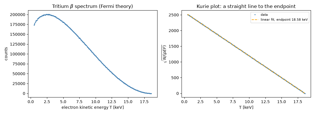
Kurie-plot endpoint: 18.585 keV  (input 18.591 keV)

A neutrino mass would bend the line

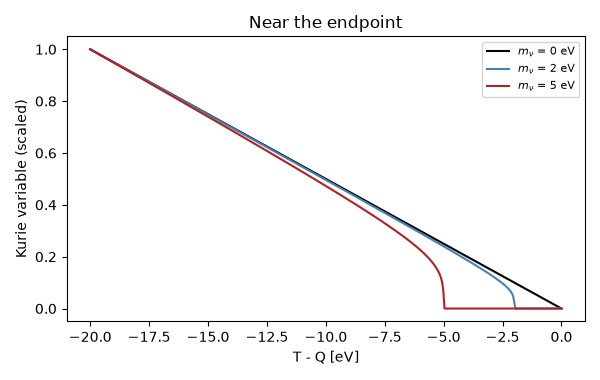
Fermi noted that the spectrum’s shape near the endpoint depends on the neutrino mass. Zooming in on the last 20 eV: a massive neutrino pulls the endpoint in by \(m_\nu\) and bends the Kurie plot down. Tritium endpoint experiments (KATRIN today) use exactly this.

T_end = np.linspace(Q_H3 - 20e-6, Q_H3, 400)
fig2, ax3 = plt.subplots(figsize=(6, 3.8))
for m_nu, color in [(0.0, "k"), (2e-6, "steelblue"), (5e-6, "firebrick")]:
    K = np.sqrt(spectrum(T_end, Q_H3, 2, m_nu) / (fermi_function(2, T_end) * np.sqrt((T_end + m_e) ** 2 - m_e**2) * (T_end + m_e)))
    ax3.plot((T_end - Q_H3) * 1e6, K / K.max(), color=color, label=rf"$m_\nu$ = {m_nu * 1e6:.0f} eV")
ax3.set_xlabel("T - Q [eV]")
ax3.set_ylabel("Kurie variable (scaled)")
ax3.set_title("Near the endpoint")
ax3.legend(fontsize=8)
fig2.tight_layout()

Sargent’s rule: the rate grows as \(Q^5\)

Integrating the spectrum (Fermi function set to 1 to isolate phase space) gives the total rate. For \(Q\gg m_e\) the log-log slope approaches 5.

Q_values = np.geomspace(0.05, 20.0, 25)
rates = []
for Qv in Q_values:
    Tg = np.linspace(1e-6, Qv, 4000)
    E = Tg + m_e
    rates.append(trapezoid(np.sqrt(E**2 - m_e**2) * E * (Qv - Tg) ** 2, Tg))
rates = np.array(rates)
slope_high = np.polyfit(np.log(Q_values[-6:]), np.log(rates[-6:]), 1)[0]
print(f"d ln(rate) / d ln(Q) for Q = 5-20 MeV: {slope_high:.2f}  (Fermi/Sargent: 5)")

fig3, ax4 = plt.subplots(figsize=(6, 3.8))
ax4.loglog(Q_values, rates, "o", color="steelblue", ms=4, label="integrated phase space")
ax4.loglog(Q_values, rates[-1] * (Q_values / Q_values[-1]) ** 5, "--", color="orange", label=r"$\propto Q^5$")
ax4.set_xlabel("endpoint energy Q [MeV]")
ax4.set_ylabel("total decay rate (arb.)")
ax4.set_title("Sargent's rule from Fermi's theory")
ax4.legend(fontsize=8)
fig3.tight_layout()

plt.show()

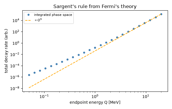
d ln(rate) / d ln(Q) for Q = 5-20 MeV: 4.79  (Fermi/Sargent: 5)

Check

Neutron endpoint 0.782 MeV; the Kurie plot is straight up to the tritium endpoint 18.59 keV; and the integrated rate approaches Sargent’s Q^5.

assert abs(Q_n - 0.7823) < 1e-3
assert abs(-b / a - Q_H3) < 0.05e-3
assert 4.5 < slope_high <= 5.0