Weibel filamentation: growing current filaments from temperature anisotropy

Erich Weibel (1959) found that a plasma whose velocity distribution is anisotropic (\(T_\perp>T_\parallel\), no bulk streaming at all) is unstable to a purely growing transverse electromagnetic mode – no beam, density gradient, or external field required. Burton Fried, the same year, supplied the physical mechanism: a random transverse magnetic fluctuation curves particle orbits enough to bunch them into current channels, and the growing channel current reinforces exactly the fluctuation that curved the orbits into existence – a self-sustaining feedback loop with no threshold.

For a wavevector \(k\) transverse to the anisotropy axis, the non-relativistic, cold-parallel-limit linear growth rate is

\[\gamma(k)^2 = \omega_{pe}^2\left(\frac{T_\perp}{T_\parallel}-1\right) - k^2c^2,\]

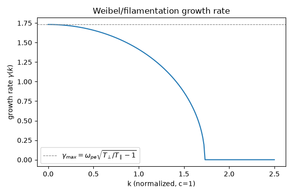
purely growing (\(\gamma\) real) for \(T_\perp>T_\parallel\) up to the cutoff wavenumber \(k_{max}=(\omega_{pe}/c)\sqrt{T_\perp/T_\parallel-1}\), beyond which the field’s own magnetic tension (the \(k^2c^2\) term) overcomes the free energy the anisotropy supplies. Growth is fastest at \(k=0\), where \(\gamma_{max}=\omega_{pe}\sqrt{T_\perp/T_\parallel-1}\).

weibel_growth_rate() evaluates the linear growth rate directly, and simulate_weibel_filamentation() superposes a spectrum of independently growing transverse-current Fourier modes – exact linear theory standing in for a full 2D-in-velocity electromagnetic PIC code – to show the real-space current filaments forming.

import matplotlib.pyplot as plt
import numpy as np
from matplotlib.colors import SymLogNorm

import physicskit as pk

Growth rate vs. wavenumber, for a strongly anisotropic population

Growth is fastest at k=0 and cuts off entirely beyond a wavenumber set by the anisotropy, where the field’s own magnetic tension overcomes the free energy the anisotropy supplies.

wpe, aniso = 1.0, 4.0
k0, gamma_max = pk.plasma.weibel_fastest_growing_mode(wpe, aniso)
k_vals = np.linspace(0.0, 2.5, 200)
gamma_vals = pk.plasma.weibel_growth_rate(k_vals, wpe=wpe, temperature_anisotropy=aniso, c=1.0)

fig, ax = plt.subplots(figsize=(6, 4))
ax.plot(k_vals, gamma_vals)
ax.axhline(gamma_max, color="gray", linestyle="--", linewidth=0.8, label=r"$\gamma_{max}=\omega_{pe}\sqrt{T_\perp/T_\parallel-1}$")
ax.set_xlabel("k (normalized, c=1)")
ax.set_ylabel(r"growth rate $\gamma(k)$")
ax.set_title("Weibel/filamentation growth rate")
ax.legend()
fig.tight_layout()

plt.show()

Filament growth from seeded current modes

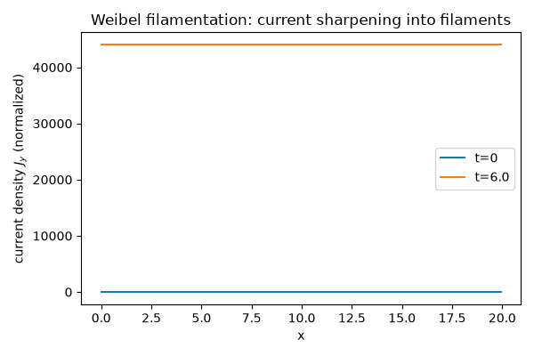
A spectrum of transverse-current Fourier modes, each growing at its own linear rate, sharpens from small random noise into distinct current filaments as the longer-wavelength (faster-growing) modes overtake the rest.

x = np.linspace(0, 20.0, 256, endpoint=False)
t = np.linspace(0, 6.0, 60)
J = pk.plasma.simulate_weibel_filamentation(x, t, wpe, aniso, n_modes=10, seed=0)

fig, ax = plt.subplots(figsize=(6, 4))
ax.plot(x, J[0], label="t=0")
ax.plot(x, J[-1], label=f"t={t[-1]:.1f}")
ax.set_xlabel("x")
ax.set_ylabel(r"current density $J_y$ (normalized)")
ax.set_title("Weibel filamentation: current sharpening into filaments")
ax.legend()
fig.tight_layout()

plt.show()

The full space-time picture

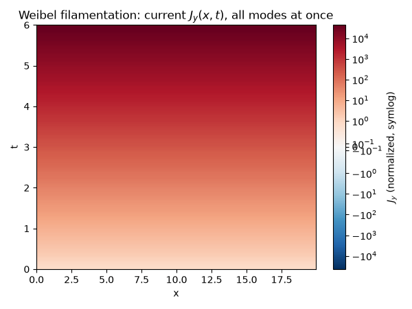
The two snapshots above are just the first and last rows of the same J array already computed; stacking every row into one image (no extra simulation needed) shows the longer-wavelength, faster-growing modes overtaking the shorter ones continuously in real space, rather than only at the two endpoints. A symmetric-log color scale is needed because the exponential growth spans many decades between the seeded noise at t=0 and the saturated filaments at the final time.

fig, ax = plt.subplots(figsize=(6, 4.5))
vmax = np.max(np.abs(J))
norm = SymLogNorm(linthresh=max(np.abs(J[0]).max(), 1e-6), vmin=-vmax, vmax=vmax)
im = ax.imshow(J, origin="lower", aspect="auto", extent=[x[0], x[-1], t[0], t[-1]], cmap="RdBu_r", norm=norm)
fig.colorbar(im, ax=ax, label=r"$J_y$ (normalized, symlog)")
ax.set_xlabel("x")
ax.set_ylabel("t")
ax.set_title("Weibel filamentation: current $J_y(x,t)$, all modes at once")
fig.tight_layout()

plt.show()

Animating the filaments forming

anim = pk.plasma.animate_weibel_filamentation(x, t, wpe, aniso, n_modes=10, seed=0)

plt.show()