Langmuir waves: electron density ringing at the plasma frequency

Irving Langmuir (1928) discovered that a plasma’s electron gas resonates at a sharply defined natural frequency: displace the electrons and their own restoring electric field snaps them back, overshoots, and rings, exactly like a mass on a spring built from nothing but the plasma’s own charge density. langmuir_wave_ic() seeds a particle-in-cell plasma with a sinusoidal displacement and a coherent velocity kick,

\[\delta x = \frac{\alpha}{k}\sin(kx_0), \qquad \delta v = \frac{\alpha\,\omega_{pe}}{k}\sin(kx_0),\]

giving the density perturbation \(n(x)\approx n_0\big(1-\alpha\cos(kx)\big)\), which then rings in place as a standing wave at \(\omega\approx\omega_{pe}\). The thermal spread here is small (\(k\lambda_D \ll 1\)), so Landau damping is negligible and the oscillation persists for many periods – in contrast to the warmer plasma of the Landau-damping example, where \(k\lambda_D\) is large enough for resonant electrons to drain the wave.

pic_simulate() evolves this initial condition exactly as it does for Landau damping and the two-stream instability: the same particles, the same field solve, no wave equation assumed anywhere.

import matplotlib.pyplot as plt
import numpy as np

import physicskit as pk

A single-mode density-and-velocity perturbation

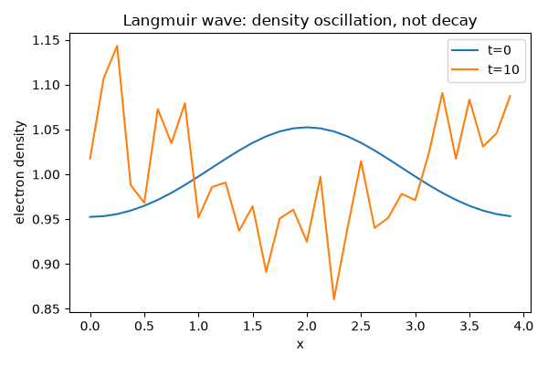
k * lambda_D is kept small (cold, slow thermal spread) so the wave is only weakly Landau-damped and rings for many periods instead of decaying.

k_mode, v_th = 2 * np.pi / 4.0, 0.05
L = 4.0
x0, v0 = pk.plasma.langmuir_wave_ic(4000, L=L, k_mode=k_mode, alpha=0.05, v_th=v_th, seed=0)

The density oscillates in place at (approximately) omega_pe

Depositing the particle positions onto a grid at several times during the run shows the same standing-wave pattern recurring, rather than decaying, because both the density and velocity perturbations carry the correct linear-theory phase relationship.

ng = 32
result = pk.plasma.pic_simulate(x0, v0, L=L, ng=ng, dt=0.05, steps=200)
x_grid = np.linspace(0.0, L, ng, endpoint=False)
n_initial = pk.plasma.deposit_number_density(x0, L, ng)
n_final = pk.plasma.deposit_number_density(result["x"], L, ng)

fig, ax = plt.subplots(figsize=(6, 4))
ax.plot(x_grid, n_initial, label="t=0")
ax.plot(x_grid, n_final, label="t=10")
ax.set_xlabel("x")
ax.set_ylabel("electron density")
ax.set_title("Langmuir wave: density oscillation, not decay")
ax.legend()
fig.tight_layout()

plt.show()

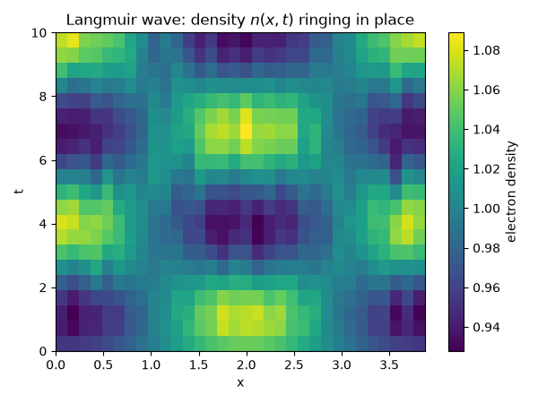
The full space-time ringing pattern

The before/after snapshot above could just as easily be a half-period phase flip rather than genuine ringing; re-running the same pic_simulate() from the identical initial condition out to a sequence of intermediate step counts and depositing the density at each shows the standing pattern recurring periodically at (approximately) omega_pe, rather than the density structure decaying, translating, or growing. A larger particle count than the two-snapshot comparison above is used here purely to keep discreteness noise from swamping the pattern across so many rows.

x0_dense, v0_dense = pk.plasma.langmuir_wave_ic(150000, L=L, k_mode=k_mode, alpha=0.05, v_th=v_th, seed=0)
snapshot_steps = np.linspace(0, 200, 21, dtype=int)
density_history = np.empty((len(snapshot_steps), ng))
for i, s in enumerate(snapshot_steps):
    if s == 0:
        density_history[i] = pk.plasma.deposit_number_density(x0_dense, L, ng)
    else:
        snap = pk.plasma.pic_simulate(x0_dense, v0_dense, L=L, ng=ng, dt=0.05, steps=int(s))
        density_history[i] = pk.plasma.deposit_number_density(snap["x"], L, ng)

fig, ax = plt.subplots(figsize=(6, 4.5))
im = ax.imshow(
    density_history,
    origin="lower",
    aspect="auto",
    extent=[x_grid[0], x_grid[-1], 0.0, snapshot_steps[-1] * 0.05],
    cmap="viridis",
)
fig.colorbar(im, ax=ax, label="electron density")
ax.set_xlabel("x")
ax.set_ylabel("t")
ax.set_title("Langmuir wave: density $n(x,t)$ ringing in place")
fig.tight_layout()

plt.show()

Animating the standing-wave oscillation

anim = pk.plasma.animate_langmuir_wave(x0, v0, L=L, ng=ng, dt=0.05, steps_per_frame=4, n_frames=60)

plt.show()