Alfven waves and the magnetosonic wave-speed diagram

In 1942, Hannes Alfven proposed that a magnetized, highly conducting fluid should support a wave nobody had previously imagined: magnetic field lines, frozen into the plasma by its high conductivity, behave like strings under tension \(B^2/\mu_0\), plucked sideways by the fluid’s own inertia. The result – the Alfven wave – travels at \(v_A = B/\sqrt{\mu_0\rho}\), purely transverse and non-compressive, and founded magnetohydrodynamics (MHD) as a discipline treating the plasma as a single conducting fluid.

alfven_speed() computes \(v_A\) directly; magnetosonic_speeds() extends the idea to the compressive fast and slow modes that appear once plasma pressure (sound speed \(c_s=\sqrt{\gamma p/\rho}\)) is added back into the picture. At propagation angle \(\theta\) to \(\mathbf{B}_0\) the two compressive MHD normal modes solve

\[v_{f,s}^2 = \frac{1}{2}\left[(v_A^2+c_s^2) \pm \sqrt{(v_A^2+c_s^2)^2 - 4v_A^2c_s^2\cos^2\theta}\right],\]

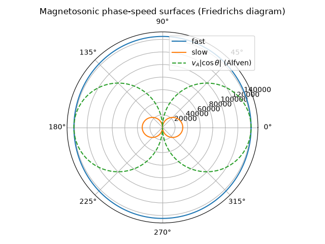
which reduce to \(\max(v_A,c_s)\)/\(\min(v_A,c_s)\) along \(\mathbf{B}_0\) (\(\theta=0\)) and to a purely compressive \(\sqrt{v_A^2+c_s^2}\) (fast) with a vanishing slow mode across it (\(\theta=\pi/2\)).

import matplotlib.pyplot as plt
import numpy as np

import physicskit as pk

A magnetized coronal-loop-like plasma

B, rho = 0.02, 1.6e-8
vA = pk.plasma.alfven_speed(B, rho)
cs = pk.plasma.sound_speed(gamma=5 / 3, p=10.0, rho=rho)

Fast/slow magnetosonic speeds at every angle to B0

Alfven’s own purely transverse wave is the limit these two compressive modes build on: it sits exactly between them, along B0.

theta = np.linspace(0, 2 * np.pi, 400)
vf, vs = zip(*[pk.plasma.magnetosonic_speeds(vA, cs, th) for th in theta], strict=True)

fig, ax = plt.subplots(subplot_kw={"projection": "polar"})
ax.plot(theta, vf, label="fast")
ax.plot(theta, vs, label="slow")
ax.plot(theta, vA * np.abs(np.cos(theta)), "--", label=r"$v_A|\cos\theta|$ (Alfven)")
ax.set_title("Magnetosonic phase-speed surfaces (Friedrichs diagram)")
ax.legend(loc="upper right")
fig.tight_layout()

plt.show()

A plucked field line: the Alfven pulse propagating and splitting

Alfven’s own analogy is a field line under tension, plucked sideways. Releasing a transverse pulse from rest and evolving the linearized 1D ideal-MHD induction and momentum equations,

\[\partial_t B_y = B_0\,\partial_x v_y, \qquad \rho_0\,\partial_t v_y = \frac{B_0}{\mu_0}\,\partial_x B_y,\]

which combine into the non-dispersive wave equation \(\partial_t^2 B_y = v_A^2\partial_x^2 B_y\), shows it split exactly in half and travel outward at \(\pm v_A\) in each direction – the picture reproduced dynamically rather than just asserted.

x = np.linspace(-20, 20, 256, endpoint=False)
By0, vy0 = pk.plasma.alfven_wave_pulse_ic(x, x0=0.0, width=1.0, amplitude=0.1)

anim = pk.plasma.animate_alfven_wave(By0, vy0, x, dt=0.01, steps_per_frame=20, n_frames=40, B0=1.0, rho0=1.0)

plt.show()