The Sweet-Parker reconnection-rate bottleneck

Peter Sweet and Eugene Parker (1957-1958) proposed the first quantitative model of magnetic reconnection: oppositely directed field lines are driven together into a long, thin resistive current sheet of length \(L\), where finite conductivity \(\eta\) finally lets them break and reconnect. The relevant dimensionless control parameter is the Lundquist number \(S=Lv_A/\eta\), the ratio of the resistive diffusion time \(L^2/\eta\) to the Alfven crossing time \(L/v_A\). Mass conservation through the sheet’s narrow exit throttles the whole process to

\[\frac{v_{in}}{v_A} = S^{-1/2}, \qquad \delta = \frac{L}{\sqrt{S}},\]

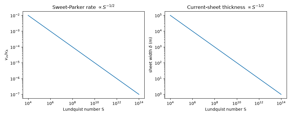
a reconnection rate and current-sheet thickness that both fall as \(S^{-1/2}\) – for solar-flare conditions (\(S\sim10^{12}\)), millions of times slower than flares are observed to release their energy, a discrepancy that stood as an open problem until Petschek’s 1964 revision (Petschek vs. Sweet-Parker reconnection).

lundquist_number() and sweet_parker_rate() / sweet_parker_layer_width() reproduce the model’s scaling laws directly. Beyond the steady-state scaling laws, simulate_reconnection() time-steps an actual X-point reconnecting – a generic kinematic resistive-induction model closer in spirit to Sweet-Parker’s diffusion-throttled picture than to Petschek’s localized-shock geometry.

import matplotlib.pyplot as plt
import numpy as np

import physicskit as pk

Sweep the Lundquist number from laboratory to solar-flare scale

At S ~ 1e12 (solar flare conditions) the predicted inflow speed is millions of times slower than observed flare energy release.

S_vals = np.logspace(4, 14, 50)
rate = np.array([pk.plasma.sweet_parker_rate(S) for S in S_vals])
width = np.array([pk.plasma.sweet_parker_layer_width(1e7, S) for S in S_vals])

fig, axes = plt.subplots(1, 2, figsize=(10, 4))
axes[0].loglog(S_vals, rate)
axes[0].set_xlabel("Lundquist number S")
axes[0].set_ylabel(r"$v_{in}/v_A$")
axes[0].set_title(r"Sweet-Parker rate $\propto S^{-1/2}$")

axes[1].loglog(S_vals, width)
axes[1].set_xlabel("Lundquist number S")
axes[1].set_ylabel(r"sheet width $\delta$ (m)")
axes[1].set_title(r"Current-sheet thickness $\propto S^{-1/2}$")
fig.tight_layout()

plt.show()

An actual X-point reconnecting: the kinematic resistive-induction model

The scaling laws above describe a steady-state reconnection rate; this builds the perturbed Harris current sheet the picture presumes and animates the flux function \(\psi(x,y,t)\) actually breaking and reconnecting at the X-point under the resistive induction equation

\[\partial_t\psi = \eta\nabla^2\psi - \mathbf{v}\cdot\nabla\psi,\]

with a prescribed inflow \(\mathbf{v}\) and finite resistivity \(\eta\) – exactly Faraday’s law with an Ohmic (rather than ideal) Ohm’s law, restricted to a fixed (kinematic) flow field rather than a self-consistently solved momentum equation.

psi0 = pk.plasma.reconnection_harris_ic(96, 96, Lx=20.0, Ly=20.0, sheet_width=1.0, perturbation_amplitude=0.2)

anim = pk.plasma.animate_reconnection(psi0, eta=0.15, v0=0.15, dt=0.05, steps_per_frame=8, n_frames=50, Lx=20.0, Ly=20.0, interval=100)

plt.show()