Solving the Grad-Shafranov equation for nested flux surfaces

Harold Grad and Hanan Rubin, and independently Vitalii Shafranov, derived (1958) the equation governing any static, axisymmetric magnetized-plasma equilibrium: force balance between the pressure gradient and the \(\mathbf{J}\times\mathbf{B}\) force reduces, in toroidal geometry, to a single nonlinear elliptic PDE for the poloidal flux function \(\psi(R,Z)\),

\[\Delta^*\psi = -\mu_0 R^2 p'(\psi) - FF'(\psi).\]

Every tokamak’s magnetic geometry – the nested flux surfaces confining its plasma – is, to leading order, a numerical solution of this one equation.

solve_grad_shafranov() solves the equation by successive over-relaxation for the linear (Solov’ev) source term, validated against the exact closed-form solution in solovev_particular_solution(); safety_factor_large_aspect_ratio() extracts the resulting field-line pitch.

import matplotlib.pyplot as plt
import numpy as np

import physicskit as pk

A rectangular (R, Z) grid around a linear (Solov’ev) equilibrium

Taking \(p'(\psi)\) and \(FF'(\psi)\) (the pressure and poloidal-current profiles) constant reduces the right-hand side to the linear source \(\Delta^*\psi = c_1 R^2 + c_2\), which admits the exact polynomial (Solov’ev) solution \(\psi_p = \tfrac{c_1}{8}R^4 + \tfrac{c_2}{2}Z^2\). Relaxing the full elliptic operator by SOR on a rectangular \((R, Z)\) grid, using this exact solution only for its Dirichlet boundary data, is then validated against that same exact solution everywhere inside.

R = np.linspace(0.5, 1.5, 61)
Z = np.linspace(-0.5, 0.5, 61)
c1, c2 = 1.0, -2.0

psi = pk.plasma.solve_grad_shafranov(R, Z, c1, c2)

RR, ZZ = np.meshgrid(R, Z, indexing="ij")
psi_exact = pk.plasma.solovev_particular_solution(RR, ZZ, c1, c2)
print("max |psi - psi_exact|:", np.max(np.abs(psi - psi_exact)))

fig, axes = plt.subplots(1, 2, figsize=(10, 4))
pk.plasma.plot_flux_surfaces(R, Z, psi, ax=axes[0])
axes[0].set_title("Nested poloidal flux surfaces")

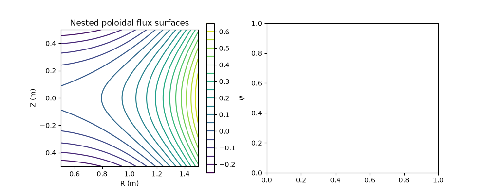
max |psi - psi_exact|: 4.989830307916554e-06

Text(0.5, 1.0, 'Nested poloidal flux surfaces')

The safety factor

In the large-aspect-ratio approximation, the safety factor

\[q \approx \frac{r B_t}{R_0 B_p}\]

counts how many times a field line winds the long way (toroidally) around the torus for each time it winds the short way (poloidally); \(q=1\) marks the sawtooth-unstable surface at the core.

r_minor = np.linspace(0.05, 0.4, 30)
q = np.array([pk.plasma.safety_factor_large_aspect_ratio(r, R0=1.0, Bt=2.0, Bp=0.2) for r in r_minor])
pk.plasma.plot_q_profile(r_minor, q, ax=axes[1])
fig.tight_layout()

plt.show()