Petschek vs. Sweet-Parker reconnection

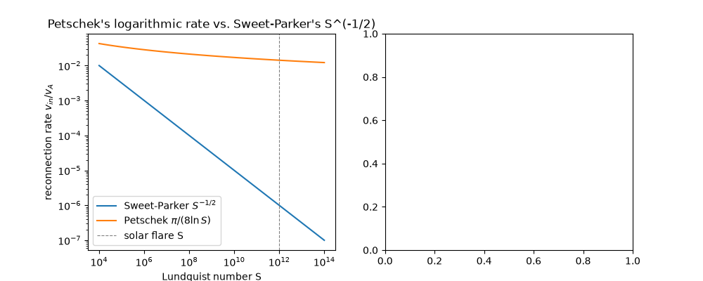
Harry Petschek (1964) proposed a resolution to the Sweet-Parker rate problem (The Sweet-Parker reconnection-rate bottleneck): if the resistive diffusion region shrinks to a small X-point rather than extending the full length of the current sheet, four standing slow-mode shocks radiating from that X-point can carry away most of the inflowing magnetic flux and energy. The resulting reconnection rate falls only logarithmically with the Lundquist number, \(v_{in}/v_A\approx\pi/(8\ln S)\), fast enough to plausibly explain solar flare and magnetospheric substorm energy-release timescales that Sweet-Parker reconnection could not.

petschek_rate() – compare directly against sweet_parker_rate() at the same Lundquist number to see the difference explode as \(S\) grows.

import matplotlib.pyplot as plt
import numpy as np

import physicskit as pk

Compare the two reconnection rates across the same S range

From laboratory to solar-flare-scale Lundquist numbers, Sweet-Parker’s S^(-1/2) collapses toward zero while Petschek’s logarithmic pi/(8 ln S) stays observationally plausible.

S_vals = np.logspace(4, 14, 50)
sp_rate = np.array([pk.plasma.sweet_parker_rate(S) for S in S_vals])
pet_rate = np.array([pk.plasma.petschek_rate(S) for S in S_vals])

fig, axes = plt.subplots(1, 2, figsize=(10, 4))
axes[0].loglog(S_vals, sp_rate, label=r"Sweet-Parker $S^{-1/2}$")
axes[0].loglog(S_vals, pet_rate, label=r"Petschek $\pi/(8\ln S)$")
axes[0].axvline(1e12, color="gray", linestyle="--", linewidth=0.8, label="solar flare S")
axes[0].set_xlabel("Lundquist number S")
axes[0].set_ylabel(r"reconnection rate $v_{in}/v_A$")
axes[0].set_title("Petschek's logarithmic rate vs. Sweet-Parker's S^(-1/2)")
axes[0].legend()

<matplotlib.legend.Legend object at 0x16b500620>

How far apart the two predictions actually are

Overlaid on a log-log rate axis, the two curves’ separation is easy to underestimate; plotting their ratio directly shows Petschek’s rate pulling ahead by many orders of magnitude precisely where it matters – solar-flare-scale Lundquist numbers.

ratio = pet_rate / sp_rate
axes[1].semilogy(S_vals, ratio, color="darkorange")
axes[1].axvline(1e12, color="gray", linestyle="--", linewidth=0.8)
s_flare_idx = np.argmin(np.abs(S_vals - 1e12))
axes[1].annotate(f"{ratio[s_flare_idx]:.0e}x at solar-flare S", (S_vals[s_flare_idx], ratio[s_flare_idx]))
axes[1].set_xscale("log")
axes[1].set_xlabel("Lundquist number S")
axes[1].set_ylabel(r"Petschek rate / Sweet-Parker rate")
axes[1].set_title("The reconnection-rate gap, made explicit")
fig.tight_layout()

plt.show()