Langmuir’s plasma frequency

In 1928, Irving Langmuir found that the electron gas in an ionized discharge tube rings at a sharply defined natural frequency: displace the electrons from the (fixed) ion background and their own restoring electric field snaps them back, overshoots, and rings, exactly like a mass on a spring built from nothing but the plasma’s own charge density,

\[\omega_p = \sqrt{\frac{n q^2}{\varepsilon_0 m}}.\]

plasma_frequency() computes this directly from the restoring-force argument, and every cold-plasma dispersion relation in physicskit.plasma.waves is built from it.

import matplotlib.pyplot as plt
import numpy as np

import physicskit as pk

From the solar wind to a tokamak core

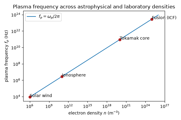
The plasma frequency spans many orders of magnitude across the densities nature and the laboratory produce it at.

labels = ["Solar wind", "Ionosphere", "Fusion (ICF)", "Tokamak core"]
n_vals = np.array([1e6, 1e11, 1e25, 1e20])  # m^-3
omega_p = np.array([pk.plasma.plasma_frequency(n) for n in n_vals])

A dense density sweep traces out the same restoring-force scaling omega_p ~ sqrt(n) continuously between those landmarks.

n_sweep = np.logspace(6, 26, 200)
omega_p_sweep = pk.plasma.plasma_frequency(n_sweep)

fig, ax = plt.subplots(figsize=(6, 4))
ax.loglog(n_sweep, omega_p_sweep / (2 * np.pi), "-", label=r"$f_p=\omega_p/2\pi$")
ax.loglog(n_vals, omega_p / (2 * np.pi), "o", color="firebrick")
for label, n, wp in zip(labels, n_vals, omega_p, strict=True):
    ax.annotate(label, (n, wp / (2 * np.pi)))
ax.set_xlabel(r"electron density $n$ (m$^{-3}$)")
ax.set_ylabel(r"plasma frequency $f_p$ (Hz)")
ax.set_title("Plasma frequency across astrophysical and laboratory densities")
ax.legend()
fig.tight_layout()

plt.show()

Overdense vs. underdense: adding the magnetic field as a second axis

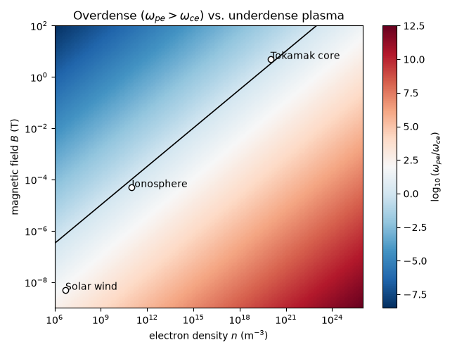
The density sweep above only tells half the story once a magnetic field is present: whether a plasma is “overdense” (\(\omega_{pe}>\omega_{ce}\), waves below \(\omega_{pe}\) are cut off) or “underdense” (\(\omega_{pe}<\omega_{ce}\), the regime cold- plasma cyclotron waves like whistlers live in) depends on both density and field strength together. Building a 2D grid of plasma_frequency() over density and cyclotron_frequency() over field strength maps that whole (n, B) parameter plane at once, with the \(\omega_{pe}=\omega_{ce}\) boundary marking the divide.

n_grid = np.logspace(6, 26, 200)
B_grid = np.logspace(-9, 2, 200)
NN, BB = np.meshgrid(n_grid, B_grid, indexing="ij")
ratio = pk.plasma.plasma_frequency(NN) / pk.plasma.cyclotron_frequency(pk.plasma.QE, pk.plasma.ME, BB)

env_labels = ["Solar wind", "Ionosphere", "Tokamak core", "Magnetar magnetosphere"]
env_n = np.array([5e6, 1e11, 1e20, 1e24])
env_B = np.array([5e-9, 5e-5, 5.0, 1e10])

fig, ax = plt.subplots(figsize=(6.5, 5))
ax.set_xscale("log")
ax.set_yscale("log")
im = ax.pcolormesh(n_grid, B_grid, np.log10(ratio.T), cmap="RdBu_r", shading="auto")
fig.colorbar(im, ax=ax, label=r"$\log_{10}(\omega_{pe}/\omega_{ce})$")
ax.contour(n_grid, B_grid, ratio.T, levels=[1.0], colors="k", linewidths=1.2)
ax.scatter(env_n, env_B, marker="o", color="black", facecolor="white", zorder=5)
for label, n, B in zip(env_labels, env_n, env_B, strict=True):
    ax.annotate(label, (n, B))
ax.set_xlim(n_grid[0], n_grid[-1])
ax.set_ylim(B_grid[0], B_grid[-1])
ax.set_xlabel(r"electron density $n$ (m$^{-3}$)")
ax.set_ylabel(r"magnetic field $B$ (T)")
ax.set_title(r"Overdense ($\omega_{pe}>\omega_{ce}$) vs. underdense plasma")
fig.tight_layout()

plt.show()