Stix’s cold-plasma dielectric tensor and the CMA diagram

Thomas Stix’s 1962 The Theory of Plasma Waves organized the zoo of magnetized cold-plasma wave modes – Alfven waves, whistlers, cyclotron waves, the ordinary and extraordinary radio-propagation modes – into a single 3x3 dielectric tensor built from each species’ plasma and cyclotron frequencies,

\[\begin{split}\mathbf{K} = \begin{pmatrix} S & -iD & 0 \\ iD & S & 0 \\ 0 & 0 & P \end{pmatrix},\end{split}\]

from which every cold-plasma dispersion relation follows as one quartic equation in the refractive index. The Clemmow-Mullaly-Allis (CMA) diagram maps the entire parameter space of that quartic onto one two-dimensional plot.

stix_parameters() builds \(S\), \(D\), \(P\) for an arbitrary multi-species plasma; cold_plasma_dispersion() solves the resulting quartic at any propagation angle, and cma_coordinates() supplies the CMA diagram’s axes.

import matplotlib.pyplot as plt
import numpy as np

import physicskit as pk

Tracing a CMA trajectory

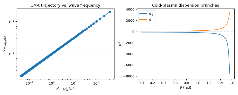
A magnetized electron-proton plasma, swept in wave frequency across the electron cyclotron resonance, traces one path on the CMA map.

n0, B0 = 1e19, 1.0
wpe = pk.plasma.plasma_frequency(n0)
wce = pk.plasma.cyclotron_frequency(pk.plasma.QE, pk.plasma.ME, B0)
omega_scan = np.linspace(0.05 * wce, 5 * wce, 300)
X, Y = pk.plasma.cma_coordinates(omega_scan, wpe, wce)

At a fixed frequency, the same species build S, D, P, and solving the quartic gives the two cold-plasma wave branches at every propagation angle to B0.

species = [(n0, -pk.plasma.QE, pk.plasma.ME), (n0, pk.plasma.QE, pk.plasma.MP)]
S, D, P = pk.plasma.stix_parameters(omega=2e9, B=B0, species=species)
theta = np.linspace(0, np.pi / 2, 200)
n2 = np.array([pk.plasma.cold_plasma_dispersion(th, S, D, P) for th in theta])

fig, axes = plt.subplots(1, 2, figsize=(10, 4))
pk.plasma.plot_cma_diagram(X, Y, ax=axes[0])
axes[0].set_title("CMA trajectory vs. wave frequency")

axes[1].plot(theta, n2[:, 0], label=r"$n^2_+$")
axes[1].plot(theta, n2[:, 1], label=r"$n^2_-$")
axes[1].axhline(0.0, color="gray", linestyle="--", linewidth=0.8)
axes[1].set_xlabel(r"$\theta$ (rad)")
axes[1].set_ylabel(r"$n^2$")
axes[1].set_title("Cold-plasma dispersion branches")
axes[1].legend()
fig.tight_layout()

plt.show()