Bloch-sphere spin dynamics

A spin-1/2 (qubit) state evolves under \(H=-(\omega/2)\sigma_z\) (a static field along z) or \(H=-(\omega_R/2)\sigma_x\) (a resonant drive along x). Since \(\sigma_z^2=\sigma_x^2=I\), the propagator has the closed form \(e^{-i\theta\sigma} = \cos\theta\, I - i\sin\theta\, \sigma\), used directly here instead of a general matrix exponential. A final section drives the same kind of two-level system with Rabi’s own closed-form resonance formula (RabiProblem), animating the Bloch vector itself as it nutates under the drive.

import matplotlib.pyplot as plt
import numpy as np

from physicskit.quantum.chapters.spin import RabiProblem
from physicskit.quantum.core.operators import sigma_x, sigma_z
from physicskit.quantum.visualizers.bloch_sphere import (
    animate_bloch_sphere,
    plot_bloch_sphere,
    state_to_bloch_trajectory,
)


def evolve(psi0, sigma, omega, t):
    """psi(t) = exp(-i*(omega/2)*sigma*t) psi0, for sigma a Pauli matrix."""
    theta = omega * t / 2
    I = np.eye(2)
    states = np.array([(np.cos(th) * I - 1j * np.sin(th) * sigma) @ psi0 for th in theta])
    return states


t = np.linspace(0, 4 * np.pi, 300)

# Larmor precession: static field along z, initial state on the equator
omega0 = 1.0
psi0_larmor = np.array([1, 1]) / np.sqrt(2)  # |+x>, on the equator
states_larmor = evolve(psi0_larmor, sigma_z, omega0, t)
traj_larmor = state_to_bloch_trajectory(states_larmor)

# Rabi oscillation: resonant drive along x, initial state |0>
omega_R = 1.0
psi0_rabi = np.array([1, 0])  # |0>, north pole
states_rabi = evolve(psi0_rabi, sigma_x, omega_R, t)
traj_rabi = state_to_bloch_trajectory(states_rabi)
P1 = np.abs(states_rabi[:, 1]) ** 2  # population in |1>

Interactive 3D Bloch-sphere trajectories

fig_larmor = plot_bloch_sphere(trajectory=traj_larmor)
fig_larmor.update_layout(title="Larmor precession: |+x> under H=-(omega/2)sigma_z")

fig_rabi = plot_bloch_sphere(trajectory=traj_rabi)
fig_rabi.update_layout(title="Rabi oscillation: |0> under H=-(omega_R/2)sigma_x")

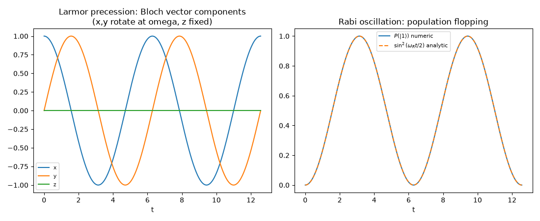
Bloch-vector components and the Rabi population curve

fig, axes = plt.subplots(1, 2, figsize=(11, 4.5))

axes[0].plot(t, traj_larmor[:, 0], label="x")
axes[0].plot(t, traj_larmor[:, 1], label="y")
axes[0].plot(t, traj_larmor[:, 2], label="z")
axes[0].set_title("Larmor precession: Bloch vector components\n(x,y rotate at omega, z fixed)")
axes[0].set_xlabel("t")
axes[0].legend(fontsize=8)

axes[1].plot(t, P1, label=r"$P(|1\rangle)$ numeric")
axes[1].plot(t, np.sin(omega_R * t / 2) ** 2, "--", label=r"$\sin^2(\omega_R t/2)$ analytic")
axes[1].set_title("Rabi oscillation: population flopping")
axes[1].set_xlabel("t")
axes[1].legend(fontsize=8)

fig.tight_layout()

print("Larmor |Bloch vector| (should stay 1):", np.round(np.linalg.norm(traj_larmor, axis=1)[:5], 6))
print("Rabi max population transfer:", P1.max())

Larmor |Bloch vector| (should stay 1): [1. 1. 1. 1. 1.]
Rabi max population transfer: 0.9999724009977419

Rabi’s resonance method: a driven two-level system, animated

RabiProblem implements Rabi’s closed-form rotating-wave-approximation propagator directly (rather than the sigma_z/sigma_x-only shortcut used above), including detuning. On resonance a “pi pulse” fully inverts the population; here animate_bloch_sphere() sweeps the Bloch vector itself, frame by frame with a matplotlib FuncAnimation, tracing the nutation from the north pole toward the south pole as the resonant drive acts – the same geometric picture Bloch introduced alongside his 1946 nuclear induction experiment.

rabi = RabiProblem(omega0=1.0, omega_d=1.0, Omega=0.5)  # on resonance (Delta=0)
t_pi = np.pi / rabi.Omega  # a resonant pi-pulse fully inverts the population
t_rabi_anim = np.linspace(0, t_pi, 60)
states_rabi_anim = rabi.state_trajectory(t_rabi_anim)
traj_rabi_anim = state_to_bloch_trajectory(states_rabi_anim)

anim = animate_bloch_sphere(traj_rabi_anim, times=t_rabi_anim)
# anim.save("rabi_bloch_sphere.gif", writer="pillow", fps=15)

print(f"population in |1> at the pi-pulse time: {rabi.excited_state_population(np.array([t_pi]))[0]:.6f}")

population in |1> at the pi-pulse time: 1.000000

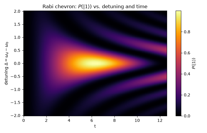
The Rabi chevron: population vs. detuning and time

Off resonance, excited_state_population() caps the population-transfer amplitude at \(\Omega^2/\Omega_R^2\) and speeds the oscillation up to the generalized Rabi frequency \(\Omega_R=\sqrt{\Delta^2+\Omega^2}\) as the drive’s detuning \(\Delta=\omega_d-\omega_0\) grows – sweeping both time and detuning traces out the “Rabi chevron”, the same 2D diagnostic pattern used to calibrate real qubit drives.

detunings = np.linspace(-2.0, 2.0, 121)
t_chevron = np.linspace(0, 4 * np.pi, 200)
chevron = np.array([RabiProblem(omega0=rabi.omega0, omega_d=rabi.omega0 + delta, Omega=rabi.Omega).excited_state_population(t_chevron) for delta in detunings])

fig_chevron, ax_chevron = plt.subplots(figsize=(7, 4.5))
im = ax_chevron.pcolormesh(t_chevron, detunings, chevron, shading="auto", cmap="inferno")
ax_chevron.set_xlabel("t")
ax_chevron.set_ylabel(r"detuning $\Delta=\omega_d-\omega_0$")
ax_chevron.set_title("Rabi chevron: $P(|1\\rangle)$ vs. detuning and time")
fig_chevron.colorbar(im, ax=ax_chevron, label=r"$P(|1\rangle)$")
fig_chevron.tight_layout()

print(f"on-resonance (Delta=0) max population: {chevron[np.argmin(np.abs(detunings))].max():.6f}")

on-resonance (Delta=0) max population: 0.999938