Bell correlations and the CHSH inequality

A textbook demonstration that quantum mechanics has no local, realistic description. Two spin-1/2 particles prepared in the entangled singlet state

\[\lvert\psi^-\rangle = \frac{\lvert01\rangle - \lvert10\rangle}{\sqrt2}\]

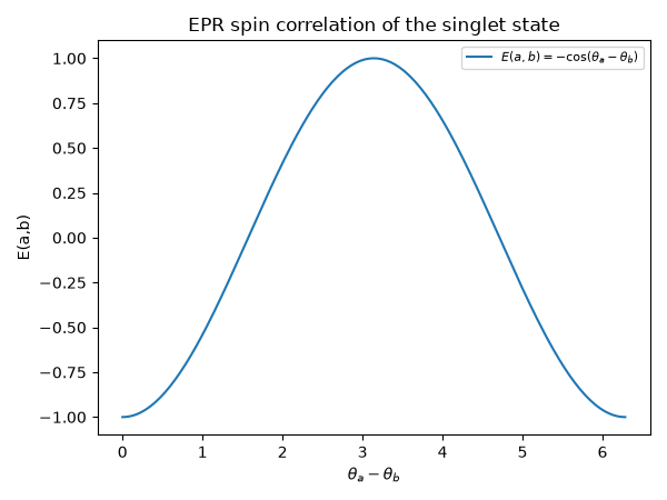
are measured along axes at angles \(\theta_a\) and \(\theta_b\) (each in the x-z plane); quantum mechanics predicts the correlation \(E(a,b) = -\cos(\theta_a - \theta_b)\), and the CHSH combination \(S = E(a,b) - E(a,b') + E(a',b) + E(a',b')\) reaches \(2\sqrt2 \approx 2.83\) at the optimal angles – exceeding the bound \(\lvert S\rvert \le 2\) that any local hidden-variable theory obeys.

import matplotlib.pyplot as plt
import numpy as np

from physicskit.quantum.chapters.entanglement import BellCorrelations

bc = BellCorrelations()
print(f"CHSH S at optimal angles: {bc.chsh_optimal():.6f}  (classical bound 2, quantum/Tsirelson bound {2 * np.sqrt(2):.6f})")

CHSH S at optimal angles: 2.828427  (classical bound 2, quantum/Tsirelson bound 2.828427)

The EPR spin correlation curve

The measured correlation \(E(a,b)\) as the relative angle \(\theta_a - \theta_b\) between the two spin analyzers is swept over a full turn.

fig, ax1 = plt.subplots(figsize=(6, 4.5))

dtheta = np.linspace(0, 2 * np.pi, 200)
E = [bc.correlation(0.0, d) for d in dtheta]
ax1.plot(dtheta, E, label=r"$E(a,b) = -\cos(\theta_a - \theta_b)$")
ax1.set_xlabel(r"$\theta_a - \theta_b$")
ax1.set_ylabel("E(a,b)")
ax1.set_title("EPR spin correlation of the singlet state")
ax1.legend(fontsize=8)
fig.tight_layout()

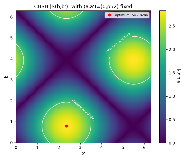
The CHSH landscape over the second observer’s two measurement angles

chsh_S() takes all four measurement angles; fixing the first observer’s pair at the optimal \((a,a')=(0,\pi/2)\) used by chsh_optimal() and sweeping the second observer’s \((b,b')\) over the full plane traces out \(|S(b,b')|\) as a 2D landscape: it peaks at the Tsirelson bound \(2\sqrt2\) exactly at \((b,b')=(\pi/4,3\pi/4)\), and a broad region around it still violates the classical bound \(|S|\le2\).

b_values = np.linspace(0, 2 * np.pi, 150)
bp_values = np.linspace(0, 2 * np.pi, 150)
S_grid = np.array([[abs(bc.chsh_S(0.0, np.pi / 2, b, bp)) for bp in bp_values] for b in b_values])

fig2, ax3 = plt.subplots(figsize=(6.5, 5.5))
im = ax3.pcolormesh(bp_values, b_values, S_grid, shading="auto", cmap="viridis")
cs = ax3.contour(bp_values, b_values, S_grid, levels=[2.0], colors="white", linewidths=1.2)
ax3.clabel(cs, fmt={2.0: "classical bound |S|=2"}, fontsize=7)
ax3.plot([3 * np.pi / 4], [np.pi / 4], "o", color="red", ms=6, label=f"optimum: S={bc.chsh_optimal():.4f}")
ax3.set_xlabel("b'")
ax3.set_ylabel("b")
ax3.set_title("CHSH |S(b,b')| with (a,a')=(0,pi/2) fixed")
ax3.legend(fontsize=8)
fig2.colorbar(im, ax=ax3, label="|S(b,b')|")
fig2.tight_layout()

print(f"max |S| over the (b,b') grid: {S_grid.max():.6f}  (Tsirelson bound {2 * np.sqrt(2):.6f})")

max |S| over the (b,b') grid: 2.828231  (Tsirelson bound 2.828427)