Planck’s quantum hypothesis and blackbody radiation

Classical physics gives every mode of the radiation field in a hot cavity the same average energy \(k_BT\). There are infinitely many short-wavelength modes, so the Rayleigh-Jeans spectrum

\[u_{RJ}(\nu) = \frac{8\pi\nu^2}{c^3}\,k_BT\]

grows without limit: the “ultraviolet catastrophe”. In December 1900 Planck assumed instead that an oscillator of frequency \(\nu\) can hold energy only in whole units \(nh\nu\). The Boltzmann average of \(nh\nu\) is then no longer \(k_BT\) but

\[\langle E\rangle = \frac{h\nu}{e^{h\nu/k_BT}-1},\]

which switches off the high-frequency modes and gives the observed spectrum. This example computes that average by summing the Boltzmann weights of each level of HarmonicOscillator, builds the spectrum from it, and recovers Wien’s displacement law and the Stefan-Boltzmann constant from physicskit.constants.

import matplotlib.pyplot as plt
import numpy as np
from scipy.integrate import quad
from scipy.optimize import minimize_scalar

from physicskit.constants import K_B, STEFAN_BOLTZMANN, C, H
from physicskit.quantum.chapters.harmonic_spin import HarmonicOscillator

Average energy of one mode: continuous vs quantized

Measured from the ground state, the oscillator’s levels are \(nh\nu\). Averaging with Boltzmann weights over the first 400 levels reproduces Planck’s closed form. At low frequency it tends to the classical \(k_BT\); at high frequency the first step, \(h\nu\), is too expensive and the mode stays empty.

osc = HarmonicOscillator(m=1.0, omega=1.0, hbar=1.0)
n = np.arange(400)
level_spacing = np.array([osc.energy(k) for k in n]) - osc.energy(0)  # in units of h nu
x_values = np.array([0.05, 0.5, 1.0, 3.0, 8.0])  # h nu / k_B T
print(f"{'h nu / kT':>10s} {'<E>/kT (sum over levels)':>26s} {'Planck':>8s} {'classical':>10s}")
for x in x_values:
    w = np.exp(-x * level_spacing)
    E_avg = np.sum(level_spacing * x * w) / np.sum(w)  # <E>/kT
    print(f"{x:10.2f} {E_avg:26.5f} {x / np.expm1(x):8.5f} {1.0:10.1f}")

h nu / kT   <E>/kT (sum over levels)   Planck  classical
     0.05                    0.97521  0.97521        1.0
     0.50                    0.77075  0.77075        1.0
     1.00                    0.58198  0.58198        1.0
     3.00                    0.15719  0.15719        1.0
     8.00                    0.00268  0.00268        1.0

The blackbody spectrum

Energy density per unit frequency: mode density \(8\pi\nu^2/c^3\) times the average energy per mode.

def planck(nu, T):
    return 8 * np.pi * H * nu**3 / C**3 / np.expm1(H * nu / (K_B * T))


def rayleigh_jeans(nu, T):
    return 8 * np.pi * nu**2 / C**3 * K_B * T


nu = np.linspace(1e12, 1.5e15, 1000)
fig, (ax1, ax2) = plt.subplots(1, 2, figsize=(11, 4))
for T, color in [(3000, "firebrick"), (4500, "darkorange"), (5800, "goldenrod")]:
    ax1.plot(nu / 1e12, planck(nu, T) * 1e15, color=color, label=f"Planck, T = {T} K")
    nu_peak = minimize_scalar(lambda v: -planck(v, T), bounds=(1e13, 1e15), method="bounded", options={"xatol": 1e6}).x
    print(f"T = {T} K: spectrum peaks at {nu_peak / 1e12:.0f} THz; nu_peak / T = {nu_peak / T:.4e} Hz/K")
ax1.plot(nu / 1e12, rayleigh_jeans(nu, 5800) * 1e15, "k--", label="Rayleigh-Jeans, 5800 K")
ax1.set_ylim(0, 1.3 * planck(nu, 5800).max() * 1e15)
ax1.set_xlabel(r"frequency $\nu$ [THz]")
ax1.set_ylabel(r"$u(\nu)$ [$10^{-15}$ J m$^{-3}$ Hz$^{-1}$]")
ax1.set_title("The ultraviolet catastrophe, avoided")
ax1.legend(fontsize=8)

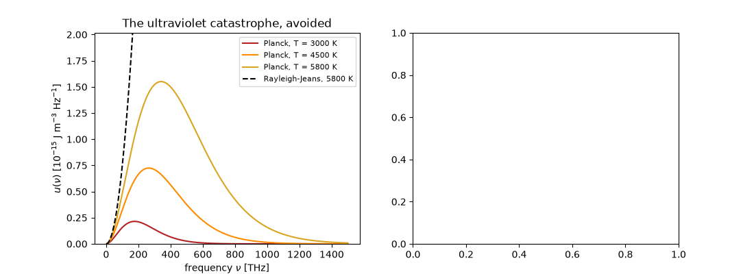
T = 3000 K: spectrum peaks at 176 THz; nu_peak / T = 5.8789e+10 Hz/K
T = 4500 K: spectrum peaks at 265 THz; nu_peak / T = 5.8789e+10 Hz/K
T = 5800 K: spectrum peaks at 341 THz; nu_peak / T = 5.8789e+10 Hz/K

<matplotlib.legend.Legend object at 0x177162780>

Wien’s displacement law and the Stefan-Boltzmann law

The peak frequency scales with \(T\): \(h\nu_{\max}=2.821\,k_BT\). Integrating over all frequencies gives \(u = aT^4\) with \(a = 8\pi^5k_B^4/(15h^3c^3) = 4\sigma/c\): Planck’s constant fixes the Stefan-Boltzmann constant.

nu_peak = minimize_scalar(lambda v: -planck(v, 5800), bounds=(1e13, 1e15), method="bounded", options={"xatol": 1e6}).x
print(f"\nWien: h nu_max / (k_B T) = {H * nu_peak / (K_B * 5800):.3f}  (theory 2.821)")
T = 5800.0
u_total = quad(lambda v: planck(v, T), 1e9, 5e16, limit=200)[0]
sigma_from_planck = u_total * C / (4 * T**4)
print(f"Stefan-Boltzmann constant from integrating Planck's law: {sigma_from_planck:.4e} W m^-2 K^-4")
print(f"CODATA value:                                            {STEFAN_BOLTZMANN:.4e} W m^-2 K^-4")

x = np.geomspace(1e-2, 20, 300)
ax2.loglog(x, x / np.expm1(x), color="steelblue", label=r"Planck: $x/(e^x-1)$")
ax2.loglog(x, np.ones_like(x), "k--", label="classical equipartition")
ax2.set_xlabel(r"$h\nu / k_BT$")
ax2.set_ylabel(r"$\langle E\rangle / k_BT$ per mode")
ax2.set_title("Quantized modes freeze out")
ax2.set_ylim(1e-8, 3)
ax2.legend(fontsize=8)
fig.tight_layout()

plt.show()

Wien: h nu_max / (k_B T) = 2.821  (theory 2.821)
Stefan-Boltzmann constant from integrating Planck's law: 5.6704e-08 W m^-2 K^-4
CODATA value:                                            5.6704e-08 W m^-2 K^-4

Check

Wien’s displacement law: h nu_max = 2.8214 k_B T; integrating Planck’s law recovers the Stefan-Boltzmann constant; the oscillator sum gives Planck’s mean energy x / (e^x - 1).

assert abs(H * nu_peak / (K_B * 5800) - 2.821439) < 1e-3
assert abs(sigma_from_planck / STEFAN_BOLTZMANN - 1) < 1e-4
for x in x_values:
    w = np.exp(-x * level_spacing)
    assert abs(np.sum(level_spacing * x * w) / np.sum(w) - x / np.expm1(x)) < 1e-6