The Born rule

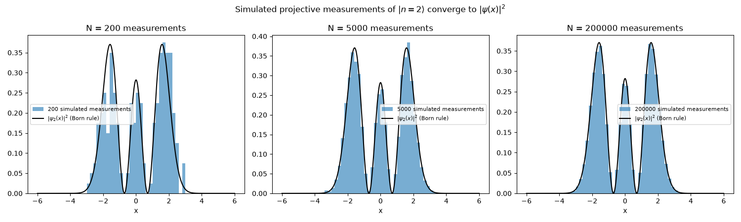
Draws simulated projective position measurements from a harmonic oscillator Fock state \(\lvert n{=}2\rangle\) via simulate_position_measurement() (inverse-CDF sampling of the Born-rule density), and shows the sample histogram converging to the analytic \(\lvert\psi_2(x)\rvert^2\) as the sample count grows.

import matplotlib.pyplot as plt
import numpy as np

from physicskit.quantum.chapters.harmonic_spin import HarmonicOscillator
from physicskit.quantum.utils.measure import simulate_position_measurement

ho = HarmonicOscillator()
n = 2
x = np.linspace(-6, 6, 2000)
psi_n = ho.eigenfunction(n, x)
density = psi_n**2

rng = np.random.default_rng(0)
sample_sizes = [200, 5000, 200000]

Histograms of simulated measurements converge to the Born-rule density

fig, axes = plt.subplots(1, len(sample_sizes), figsize=(15, 4.5))

for ax, N in zip(axes, sample_sizes):
    samples = simulate_position_measurement(x, psi_n, n_samples=N, rng=rng)
    ax.hist(samples, bins=60, range=(-6, 6), density=True, alpha=0.6, label=f"{N} simulated measurements")
    ax.plot(x, density, color="black", lw=1.5, label=r"$|\psi_2(x)|^2$ (Born rule)")
    ax.set_xlabel("x")
    ax.set_title(f"N = {N} measurements")
    ax.legend(fontsize=8)

fig.suptitle(r"Simulated projective measurements of $|n{=}2\rangle$ converge to $|\psi(x)|^2$")
fig.tight_layout()

Quantitative check: the histogram approaches the analytic density.

samples_large = simulate_position_measurement(x, psi_n, n_samples=500000, rng=rng)
hist, edges = np.histogram(samples_large, bins=100, range=(-6, 6), density=True)
centers = 0.5 * (edges[1:] + edges[:-1])
analytic = np.interp(centers, x, density)
mean_abs_err = np.mean(np.abs(hist - analytic))
print(f"mean |histogram - |psi|^2| at N=500000: {mean_abs_err:.5f}")

mean |histogram - |psi|^2| at N=500000: 0.00084

Convergence to the Born rule across Fock states and sample sizes

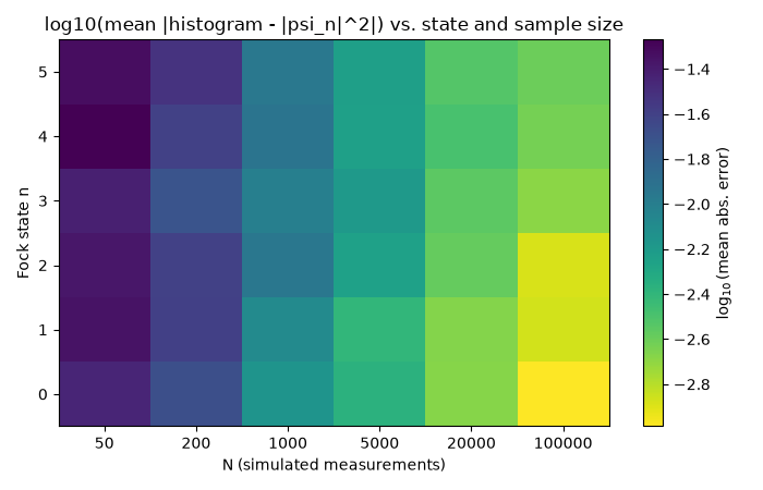
The single-state convergence above is one slice of a broader picture: simulate_position_measurement() applied to several Fock states \(|n\rangle\), each at several sample counts, shows the same histogram-vs-analytic error shrinking with \(N\) regardless of the state’s shape – a 2D map instead of a single 1D convergence curve.

n_grid = np.arange(0, 6)
N_grid = np.array([50, 200, 1000, 5000, 20000, 100000])
error_map = np.zeros((len(n_grid), len(N_grid)))
for i, n_state in enumerate(n_grid):
    psi_state = ho.eigenfunction(int(n_state), x)
    density_state = psi_state**2
    for j, N in enumerate(N_grid):
        samples = simulate_position_measurement(x, psi_state, n_samples=int(N), rng=rng)
        h, e = np.histogram(samples, bins=60, range=(-6, 6), density=True)
        c = 0.5 * (e[1:] + e[:-1])
        a = np.interp(c, x, density_state)
        error_map[i, j] = np.mean(np.abs(h - a))

fig2, ax2 = plt.subplots(figsize=(7, 4.5))
im = ax2.pcolormesh(np.arange(len(N_grid)), n_grid, np.log10(error_map), shading="auto", cmap="viridis_r")
ax2.set_xticks(np.arange(len(N_grid)))
ax2.set_xticklabels([str(N) for N in N_grid])
ax2.set_xlabel("N (simulated measurements)")
ax2.set_ylabel("Fock state n")
ax2.set_title("log10(mean |histogram - |psi_n|^2|) vs. state and sample size")
fig2.colorbar(im, ax=ax2, label=r"$\log_{10}$(mean abs. error)")
fig2.tight_layout()