The double-slit experiment, propagated in time

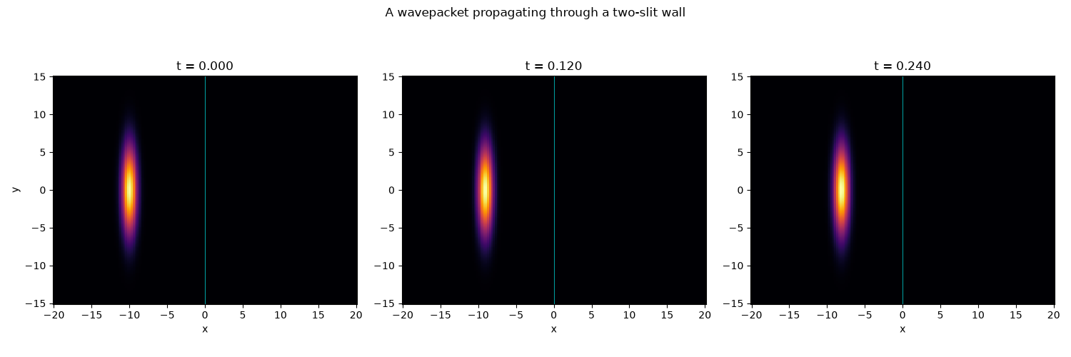
Propagates a genuine 2D Gaussian wavepacket – elongated along \(y\) so it illuminates both slits coherently – through an opaque wall pierced by two gaps (double_slit_potential()) using the FFT split-operator method (SplitOperatorSolver2D). 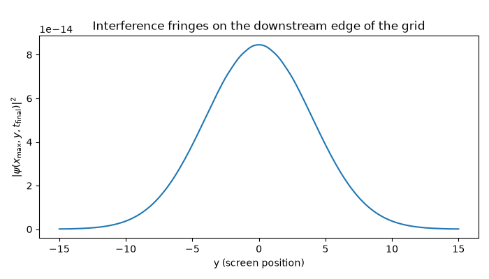Unlike the far-field Fraunhofer formula used in TwinSlit (Dispersion, twin-slit interference, and quantum revivals), the interference fringes here build up from genuine wave dynamics: the packet splits at the wall, the two emerging pieces spread and overlap downstream, and the familiar fringe pattern \(\lvert\psi_1+\psi_2\rvert^2\) emerges directly from the time-dependent Schrodinger equation – exactly the electron-at-a-time interference Jonsson observed in 1961.

import matplotlib.pyplot as plt
import numpy as np

from physicskit.quantum.chapters.wave_packets import propagate_double_slit
from physicskit.quantum.visualizers.wavefunctions import animate_density_2d

x = np.linspace(-20, 20, 160)
y = np.linspace(-15, 15, 160)

X, Y, frames, times = propagate_double_slit(
    x,
    y,
    x0=-10.0,
    k0=8.0,
    sigma_x=0.7,
    sigma_y=4.0,
    wall_x=0.0,
    slit_separation=3.0,
    slit_width=0.8,
    dt=1e-4,
    n_steps=2400,
    save_every=40,
)

dx, dy = x[1] - x[0], y[1] - y[0]
norm0 = float(np.sum(np.abs(frames[0]) ** 2)) * dx * dy
norm_end = float(np.sum(np.abs(frames[-1]) ** 2)) * dx * dy
print(f"norm conservation check: {norm0:.6f} -> {norm_end:.6f}")

norm conservation check: 1.000017 -> 1.000017

Snapshots before, during, and after the wall, and the fringe pattern building up on a downstream screen ————————————————————————–

fig, axes = plt.subplots(1, 3, figsize=(15, 5))
snapshot_idx = [0, len(frames) // 2, -1]
for ax, i in zip(axes, snapshot_idx):
    density = np.abs(frames[i]) ** 2
    ax.pcolormesh(X, Y, density, shading="auto", cmap="inferno")
    ax.axvline(0.0, color="cyan", lw=0.8, alpha=0.6)
    ax.set_title(f"t = {times[i]:.3f}")
    ax.set_xlabel("x")
    ax.set_aspect("equal")
axes[0].set_ylabel("y")
fig.suptitle("A wavepacket propagating through a two-slit wall")
fig.tight_layout()

screen_density = np.abs(frames[-1][-1, :]) ** 2  # density along the far x-edge (the "screen")
fig2, ax2 = plt.subplots(figsize=(7, 4))
ax2.plot(y, screen_density)
ax2.set_xlabel("y (screen position)")
ax2.set_ylabel(r"$|\psi(x_\mathrm{max},y,t_\mathrm{final})|^2$")
ax2.set_title("Interference fringes on the downstream edge of the grid")
fig2.tight_layout()

• 
• 

An animation of the full time propagation

animate_density_2d() renders the complex wavefunction frame by frame, phase-colored, as it passes through the wall and the two emerging wavelets interfere.

anim = animate_density_2d(X, Y, frames, times=times)
# anim.save("double_slit.gif", writer="pillow", fps=15)