Jönsson’s electron double slit: interference one electron at a time

In 1961 Claus Jönsson sent electrons through slits a micrometre apart in a thin foil and recorded the first two-slit interference fringes made by material particles. Each electron lands at one point, but the pattern they build up is \(|\psi_1+\psi_2|^2\), the interference of the amplitudes for going through either slit.

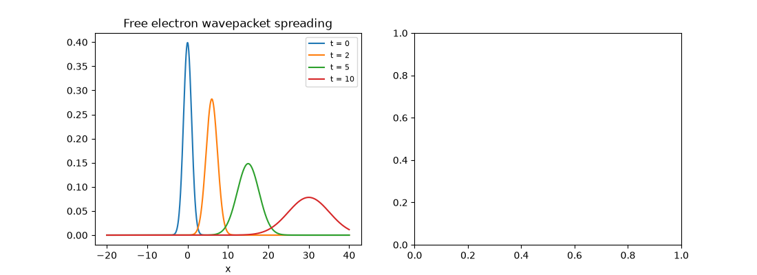
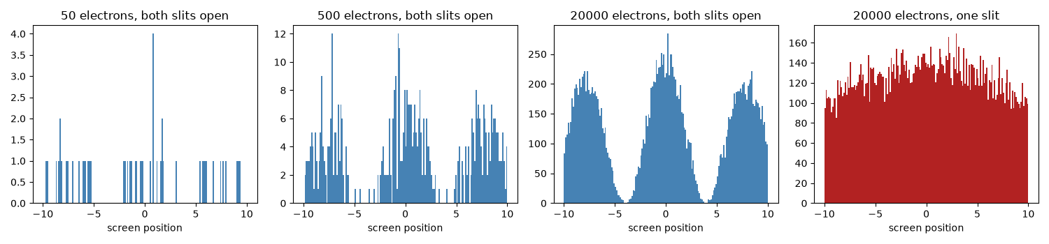
This example follows the Gaussian electron wavepacket that GaussianDispersion propagates exactly, computes the far-field two-slit pattern with TwinSlit, and then draws individual electron arrivals from it to show the fringes emerging from single, point-like detections. Blocking one slit removes them.

import matplotlib.pyplot as plt
import numpy as np
from scipy.signal import find_peaks

from physicskit.quantum.chapters.wave_packets import GaussianDispersion, TwinSlit
from physicskit.quantum.visualizers.wavefunctions import animate_density

The electron packet spreads on its way to the slits

A free Gaussian packet keeps its shape but widens as \(\sigma(t)=\sigma_0\sqrt{1+(\hbar t/2m\sigma_0^2)^2}\). The spreading is what lets a single electron’s wave cover both slits.

gd = GaussianDispersion(x0=0.0, sigma0=1.0, k0=3.0)
x1 = np.linspace(-20, 40, 1000)
fig1, (ax1, ax2) = plt.subplots(1, 2, figsize=(11, 4))
for t in [0, 2, 5, 10]:
    ax1.plot(x1, gd.density(x1, t), label=f"t = {t}")
ax1.set_xlabel("x")
ax1.set_title("Free electron wavepacket spreading")
ax1.legend(fontsize=8)

# The same exact solution, animated with its phase colour-coded: the de
# Broglie phase :math:`e^{ik_0x}` rides along the advancing centre while
# the envelope spreads.
t_anim = np.linspace(0, 6.0, 120)
x_anim = np.linspace(-20, 40, 600)
anim = animate_density(x_anim, gd.trajectory(x_anim, t_anim), times=t_anim)

• 

Two slits, and one

ts = TwinSlit(slit_separation=4.0, slit_width=0.4, k0=10.0)
y = np.linspace(-10, 10, 2000)
I_two = ts.intensity(y, screen_distance=50)
# A single open slit: the two sources merged into one (zero separation).
I_one = TwinSlit(slit_separation=0.0, slit_width=0.4, k0=10.0).intensity(y, screen_distance=50)
ax2.plot(y, I_two / I_two.max(), color="steelblue", label=r"both slits: $|\psi_1+\psi_2|^2$")
ax2.plot(y, I_one / I_one.max(), color="firebrick", ls="--", label="one slit")
peaks, _ = find_peaks(I_two)
print(f"bright fringes at y = {np.round(y[peaks], 2).tolist()}; expected spacing lambda L / d = {2 * np.pi / 10.0 * 50 / 4.0:.2f}")
ax2.set_xlabel("position on the screen")
ax2.set_ylabel("intensity (normalized)")
ax2.set_title("Far-field two-slit pattern")
ax2.legend(fontsize=8)
fig1.tight_layout()

bright fringes at y = [-7.79, -0.01, 7.79]; expected spacing lambda L / d = 7.85

Building the pattern one electron at a time

Treat the normalized intensity as the probability of each landing position and draw electrons from it. A handful look random; thousands reproduce the fringes. With one slit blocked the same number of electrons gives a single smooth band.

rng = np.random.default_rng(1961)
p_two = I_two / I_two.sum()
p_one = I_one / I_one.sum()
fig2, axes = plt.subplots(1, 4, figsize=(15, 3.5), sharey=False)
for ax, n in zip(axes[:3], (50, 500, 20000)):
    hits = rng.choice(y, size=n, p=p_two)
    ax.hist(hits, bins=160, range=(-10, 10), color="steelblue")
    ax.set_title(f"{n} electrons, both slits open")
    ax.set_xlabel("screen position")
hits_one = rng.choice(y, size=20000, p=p_one)
axes[3].hist(hits_one, bins=160, range=(-10, 10), color="firebrick")
axes[3].set_title("20000 electrons, one slit")
axes[3].set_xlabel("screen position")
fig2.tight_layout()

plt.show()

Check

Fringes spaced by lambda L / d, and a free packet’s width grows as sigma(t) = sigma0 sqrt(1 + (t / 2 sigma0^2)^2) (hbar = m = 1).

spacing = np.diff(y[peaks]).mean()
assert abs(spacing / (2 * np.pi / 10.0 * 50 / 4.0) - 1) < 0.02
x_wide = np.linspace(-30, 60, 6000)
rho = gd.density(x_wide, 5.0)
rho /= np.trapezoid(rho, x_wide)
mean = np.trapezoid(x_wide * rho, x_wide)
width = np.sqrt(np.trapezoid((x_wide - mean) ** 2 * rho, x_wide))
assert abs(mean - 3.0 * 5.0) < 1e-3
assert abs(width - np.sqrt(1 + (5.0 / 2) ** 2)) < 1e-3