Wave-packet revivals in the infinite square well

A wavepacket built from the levels of an infinite square well of width \(L\), \(E_n=n^2\pi^2\hbar^2/(2mL^2)\), disperses within a few bounces into an apparently random mess. Parker and Stroud (1986) predicted, and Yeazell, Mallalieu and Stroud (1990) observed in Rydberg atoms, that it is only dephased: because the levels grow exactly as \(n^2\), every phase \(e^{-iE_nt/\hbar}\) returns to its starting value at the revival time

\[t_\text{rev} = \frac{4mL^2}{\pi\hbar},\]

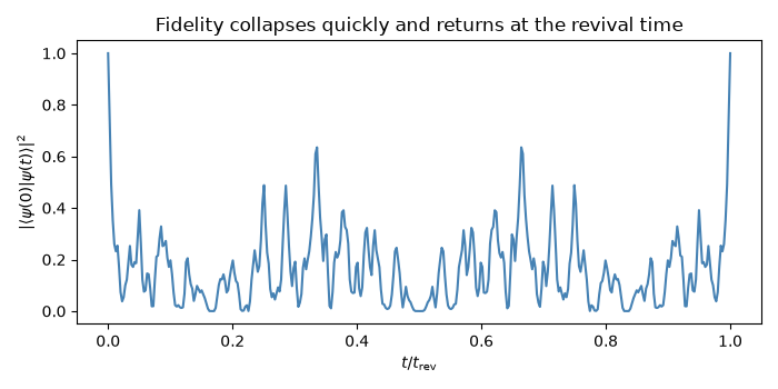
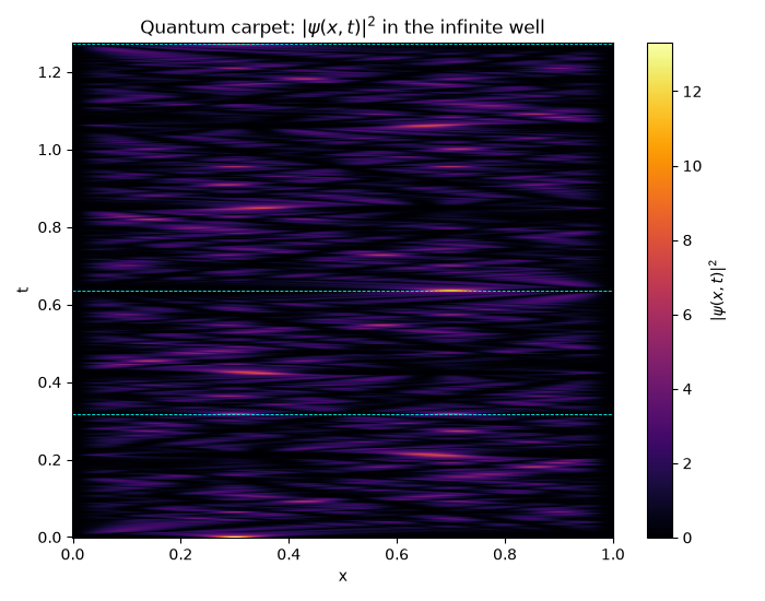
and the packet reassembles. A mirror image appears at \(t_\text{rev}/2\), and smaller copies (fractional revivals, Averbukh and Perelman 1989) at other rational fractions. This example evolves a packet with QuantumRevival, tracks its fidelity to the initial state, and draws the full space-time “quantum carpet”.

import matplotlib.pyplot as plt
import numpy as np

from physicskit.quantum.chapters.wave_packets import QuantumRevival

Collapse and revival

qr = QuantumRevival(L=1.0, n_max=300)
x = np.linspace(0, qr.L, 1500)
psi0_func = qr.gaussian_initial_state(x0=0.3, sigma=0.03)
psi0 = psi0_func(x)
coeffs = qr.eigenbasis_coefficients(psi0_func)
t_rev = qr.revival_time

fractions = [0.0, 0.05, 0.25, 0.5, 1.0]
fig, ax = plt.subplots(figsize=(7, 5))
offset = 0
for frac in fractions:
    density = np.abs(qr.wavefunction(x, frac * t_rev, coeffs)) ** 2
    ax.plot(x, density + offset, label=f"t = {frac:.2f} t_rev")
    offset += density.max() * 1.3
    fid = qr.fidelity_to_initial(x, frac * t_rev, coeffs, psi0)
    print(f"fidelity to initial state at t = {frac:.2f} t_rev: {fid:.4f}")
ax.axvline(0.0, color="black", lw=1.2)
ax.axvline(qr.L, color="black", lw=1.2)
ax.set_xlabel("x")
ax.set_yticks([])
ax.set_title("Spread out, then rebuilt: snapshots (offset vertically)")
ax.legend(fontsize=8)
fig.tight_layout()

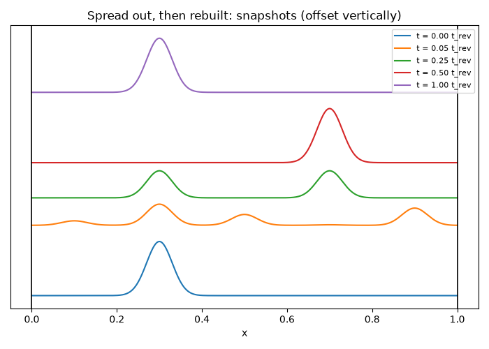
fidelity to initial state at t = 0.00 t_rev: 1.0000
fidelity to initial state at t = 0.05 t_rev: 0.3920
fidelity to initial state at t = 0.25 t_rev: 0.5000
fidelity to initial state at t = 0.50 t_rev: 0.0000
fidelity to initial state at t = 1.00 t_rev: 1.0000

Fidelity over one revival period

t_scan = np.linspace(0, t_rev, 400)
fidelity = np.array([qr.fidelity_to_initial(x, t, coeffs, psi0) for t in t_scan])
fig2, ax2 = plt.subplots(figsize=(7, 3.5))
ax2.plot(t_scan / t_rev, fidelity, color="steelblue")
ax2.set_xlabel(r"$t / t_\text{rev}$")
ax2.set_ylabel(r"$|\langle\psi(0)|\psi(t)\rangle|^2$")
ax2.set_title("Fidelity collapses quickly and returns at the revival time")
fig2.tight_layout()

A “quantum carpet”: the full space-time revival pattern

Evaluating the wavefunction on a full \((x,t)\) grid shows the web of diagonal fractional-revival ridges between the sharp replicas at \(t=0\), \(t_\text{rev}/2\) and \(t_\text{rev}\).

t_carpet = np.linspace(0, t_rev, 500)
x_carpet = np.linspace(0, qr.L, 700)
carpet = np.array([np.abs(qr.wavefunction(x_carpet, t, coeffs)) ** 2 for t in t_carpet])

fig3, ax3 = plt.subplots(figsize=(7, 5.5))
im = ax3.pcolormesh(x_carpet, t_carpet, carpet, shading="auto", cmap="inferno")
for frac in (0.25, 0.5, 1.0):
    ax3.axhline(frac * t_rev, color="cyan", ls="--", lw=0.6)
ax3.set_xlabel("x")
ax3.set_ylabel("t")
ax3.set_title(r"Quantum carpet: $|\psi(x,t)|^2$ in the infinite well")
fig3.colorbar(im, ax=ax3, label=r"$|\psi(x,t)|^2$")
fig3.tight_layout()

plt.show()

Check

Full revival at t_rev, the mirror image (no overlap) at t_rev/2, and a fractional revival into two copies (fidelity 1/2) at t_rev/4.

fid = {frac: qr.fidelity_to_initial(x, frac * t_rev, coeffs, psi0) for frac in (0.25, 0.5, 1.0)}
assert fid[1.0] > 0.999 and fid[0.5] < 1e-3 and abs(fid[0.25] - 0.5) < 1e-3