The Lindblad master equation: T1 relaxation and T2 dephasing

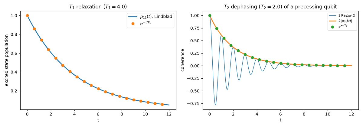
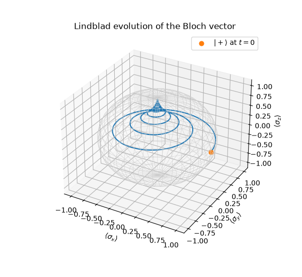
A qubit coupled to a Markovian environment obeys Lindblad’s 1976 master equation. Here solve_lindblad() evolves a qubit with energy-relaxation time \(T_1\) and coherence time \(T_2\) (collapse operators from t1_t2_collapse_operators()): the excited population decays as \(e^{-t/T_1}\), the precessing coherence \(\rho_{01}\) as \(e^{-t/T_2}\), and the Bloch vector spirals inwards towards the ground state.

import matplotlib.pyplot as plt
import numpy as np

from physicskit.quantum.chapters.open_systems import (
    amplitude_damping_kraus,
    apply_kraus,
    sigma_minus,
    solve_lindblad,
    t1_t2_collapse_operators,
)
from physicskit.quantum.core.operators import sigma_x, sigma_y, sigma_z

T1, T2, omega = 4.0, 2.0, 2 * np.pi
H = 0.5 * omega * sigma_z
t = np.linspace(0, 12, 1200)

\(T_1\): the excited state relaxes

rho_e = solve_lindblad(np.array([0, 1]), H, t1_t2_collapse_operators(T1, T2), t)

\(T_2\): an equal superposition loses its phase

plus = np.array([1, 1]) / np.sqrt(2)
rho_p = solve_lindblad(plus, H, t1_t2_collapse_operators(T1, T2), t)

fig, axes = plt.subplots(1, 2, figsize=(12, 4.2))
axes[0].plot(t, rho_e[:, 1, 1].real, lw=2, label=r"$\rho_{11}(t)$, Lindblad")
axes[0].plot(t[::60], np.exp(-t[::60] / T1), "o", label=r"$e^{-t/T_1}$")
axes[0].set_xlabel("t")
axes[0].set_ylabel("excited-state population")
axes[0].set_title(rf"$T_1$ relaxation ($T_1 = {T1}$)")
axes[0].legend()

axes[1].plot(t, 2 * rho_p[:, 0, 1].real, lw=1, label=r"$2\,\mathrm{Re}\,\rho_{01}(t)$")
axes[1].plot(t, 2 * np.abs(rho_p[:, 0, 1]), lw=2, label=r"$2|\rho_{01}(t)|$")
axes[1].plot(t[::60], np.exp(-t[::60] / T2), "o", label=r"$e^{-t/T_2}$")
axes[1].set_xlabel("t")
axes[1].set_ylabel("coherence")
axes[1].set_title(rf"$T_2$ dephasing ($T_2 = {T2}$) of a precessing qubit")
axes[1].legend(fontsize=8)
fig.tight_layout()

The Bloch vector spirals to the ground state

Relaxation shrinks the transverse components at rate \(1/T_2\) while the longitudinal one returns to \(\langle\sigma_z\rangle = +1\) (\(|0\rangle\) is the ground state) at rate \(1/T_1\).

bloch = np.array([np.einsum("ij,tji->t", s, rho_p).real for s in (sigma_x, sigma_y, sigma_z)])
fig2 = plt.figure(figsize=(6, 5.5))
ax3 = fig2.add_subplot(projection="3d")
u, v = np.mgrid[0 : 2 * np.pi : 40j, 0 : np.pi : 20j]
ax3.plot_wireframe(np.cos(u) * np.sin(v), np.sin(u) * np.sin(v), np.cos(v), color="0.8", lw=0.4)
ax3.plot(*bloch, color="C0", lw=1.5)
ax3.scatter(*bloch[:, 0], color="C1", s=40, label=r"$|+\rangle$ at $t=0$")
ax3.set_xlabel(r"$\langle\sigma_x\rangle$")
ax3.set_ylabel(r"$\langle\sigma_y\rangle$")
ax3.set_zlabel(r"$\langle\sigma_z\rangle$")
ax3.set_title("Lindblad evolution of the Bloch vector")
ax3.legend()

<matplotlib.legend.Legend object at 0x34fb9ca40>

The integrated dynamics is a quantum channel

Pure decay at rate \(\Gamma\) for a time \(t\) is exactly the amplitude-damping channel with \(\gamma = 1 - e^{-\Gamma t}\): the Lindblad semigroup is a family of completely positive, trace-preserving maps.

Gamma, t_c = 1 / T1, 2.5
rho0 = np.array([[0.3, 0.2 - 0.1j], [0.2 + 0.1j, 0.7]])
rho_lindblad = solve_lindblad(rho0, np.zeros((2, 2)), [np.sqrt(Gamma) * sigma_minus()], np.array([0.0, t_c]))[-1]
rho_kraus = apply_kraus(rho0, amplitude_damping_kraus(1 - np.exp(-Gamma * t_c)))
print("max |Lindblad - Kraus| =", np.abs(rho_lindblad - rho_kraus).max())

max |Lindblad - Kraus| = 0.0

Check

Populations relax as e^(-t/T1), coherences as e^(-t/T2); the Lindblad solution of amplitude damping equals the Kraus map with gamma = 1 - e^(-Gamma t).

np.testing.assert_allclose(rho_e[:, 1, 1].real, np.exp(-t / T1), atol=1e-6)
np.testing.assert_allclose(2 * np.abs(rho_p[:, 0, 1]), np.exp(-t / T2), atol=1e-6)
assert np.abs(rho_lindblad - rho_kraus).max() < 1e-8