Quantum trajectories: the Monte Carlo wavefunction method

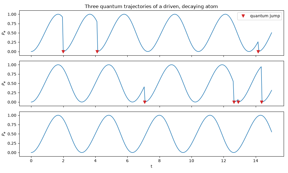
Dalibard, Castin and Molmer (1992) showed that a Lindblad master equation can be unravelled into stochastic pure-state trajectories: each evolves under a non-Hermitian effective Hamiltonian and is interrupted by random quantum jumps. Here QuantumTrajectories simulates a resonantly driven, decaying two-level atom (resonance fluorescence). Single trajectories show Rabi flopping cut short by photon emissions; their average reproduces the Lindblad density matrix.

import matplotlib.pyplot as plt
import numpy as np

from physicskit.quantum.chapters.open_systems import QuantumTrajectories, sigma_minus, solve_lindblad
from physicskit.quantum.core.operators import sigma_x

Omega, gamma = 2.0, 0.4
H = 0.5 * Omega * sigma_x
c_ops = [np.sqrt(gamma) * sigma_minus()]
t = np.linspace(0, 15, 301)
P_e = np.diag([0.0, 1.0])

res = QuantumTrajectories(H, c_ops).run(np.array([1, 0]), t, n_traj=2000, dt=0.005, rng=np.random.default_rng(0))
rho_exact = solve_lindblad(np.array([1, 0]), H, c_ops, t)

Individual trajectories jump

Each emitted photon (a jump \(\psi \to \sigma_-\psi\), marked by a dot) resets the atom to the ground state, after which Rabi flopping restarts.

pops = res.expectation(P_e, average=False)
fig, axes = plt.subplots(3, 1, figsize=(10, 6), sharex=True)
for ax, k in zip(axes, range(3)):
    ax.plot(t, pops[k], lw=1.3)
    ax.plot(res.jump_times[k], np.zeros_like(res.jump_times[k]), "v", color="C3", ms=7, label="quantum jump")
    ax.set_ylabel(r"$P_e$")
    ax.set_ylim(-0.1, 1.1)
axes[0].legend(loc="upper right")
axes[0].set_title("Three quantum trajectories of a driven, decaying atom")
axes[-1].set_xlabel("t")
fig.tight_layout()

The ensemble average is the Lindblad solution

fig2, ax2 = plt.subplots(figsize=(10, 4))
for n in (20, 200, 2000):
    ax2.plot(t, pops[:n].mean(axis=0), lw=1, label=f"average of {n} trajectories")
ax2.plot(t, rho_exact[:, 1, 1].real, "k--", lw=2, label="Lindblad master equation")
ax2.axhline(Omega**2 / (gamma**2 + 2 * Omega**2), color="0.5", ls=":", label="steady state")
ax2.set_xlabel("t")
ax2.set_ylabel("excited-state population")
ax2.set_title("Averaging quantum trajectories recovers the density matrix")
ax2.legend(fontsize=8)
fig2.tight_layout()

err = np.abs(res.density_matrices()[:, 1, 1] - rho_exact[:, 1, 1]).max()
print(f"max deviation from Lindblad with 2000 trajectories: {err:.3f} (1/sqrt(N) = {1 / np.sqrt(2000):.3f})")

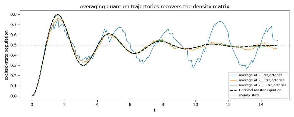
max deviation from Lindblad with 2000 trajectories: 0.018 (1/sqrt(N) = 0.022)

Waiting-time statistics

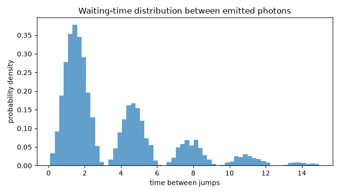
The intervals between successive jumps (photon emissions) are the delays measured in photon-counting experiments; none are near zero because an atom just reset to its ground state cannot emit again immediately – photon antibunching.

waits = np.concatenate([np.diff(np.r_[0.0, j]) for j in res.jump_times])
fig3, ax3 = plt.subplots(figsize=(7, 4))
ax3.hist(waits, bins=60, density=True, alpha=0.7)
ax3.set_xlabel("time between jumps")
ax3.set_ylabel("probability density")
ax3.set_title("Waiting-time distribution between emitted photons")
fig3.tight_layout()

Check

The trajectory average reproduces the master equation within its statistical error, and the driven two-level atom settles at the resonance-fluorescence steady state rho_ee = (Omega^2/4) / (Omega^2/2 + gamma^2/4).

assert err < 3 / np.sqrt(2000)
rho_ee_ss = (Omega**2 / 4) / (Omega**2 / 2 + gamma**2 / 4)
assert abs(rho_exact[-50:, 1, 1].real.mean() - rho_ee_ss) < 0.01