Bound states via the matrix Numerov solver

Solves and plots the low-lying eigenstates of an asymmetric step well, a finite square well (with its evanescent tails), and the gravitational “quantum bouncer” – and cross-checks the bouncer’s numerically computed energies against the exact Airy-function zeros. Each panel shows the potential shape \(V(x)\) (black), the energy levels (dashed lines), and the eigenfunctions \(\psi_n(x)\) offset to sit at their own energy.

import matplotlib.pyplot as plt
import numpy as np

from physicskit.quantum.chapters.potentials import (
    FiniteSquareWell,
    airy_bouncer_energies,
    asymmetric_well_states,
    gravitational_bouncer_states,
)
from physicskit.quantum.core.eigensolvers import asymmetric_step_well, linear_gravitational_well


def plot_well(ax, x, V, energies, wavefunctions, scale, title, xlabel="x"):
    ax.plot(x, V, color="black", lw=1.2, label="V(x)", zorder=1)
    for n in range(len(energies)):
        ax.axhline(energies[n], color="gray", lw=0.5, ls=":", zorder=0)
        ax.plot(x, energies[n] + scale * wavefunctions[n], lw=1.5, label=f"n={n}", zorder=2)
    ax.set_title(title)
    ax.set_xlabel(xlabel)
    ax.set_ylabel("energy / psi_n(x) (offset)")

Asymmetric step well, finite square well, and the gravitational bouncer

fig, axes = plt.subplots(1, 3, figsize=(15, 4.5))

# Asymmetric step well: wavefunctions decay at different rates into the
# left vs. right forbidden regions.
asym = asymmetric_well_states(n_states=4)
V_asym = asymmetric_step_well(width=2.0, V_left=40.0, V_right=15.0)(asym.x)
plot_well(axes[0], asym.x, V_asym, asym.energies, asym.wavefunctions, scale=4, title="Asymmetric step well\n(unequal decay left/right)")
axes[0].set_ylim(-2, 18)
axes[0].legend(fontsize=7, ncol=2)

# Finite square well: bound states plus evanescent tails outside the well.
fsw = FiniteSquareWell(V0=20.0, width=2.0)
bound = fsw.bound_states(n_states=6)
V_fsw = np.where(np.abs(bound.x) <= fsw.width / 2, -fsw.V0, 0.0)
plot_well(
    axes[1], bound.x, V_fsw, bound.energies, bound.wavefunctions, scale=3, title=f"Finite square well\n({len(bound.energies)} bound states, evanescent tails)"
)
axes[1].axvline(-1.0, color="gray", ls="--", lw=0.8)
axes[1].axvline(1.0, color="gray", ls="--", lw=0.8)
axes[1].set_ylim(-22, 5)

# Gravitational quantum bouncer: V(x) = alpha*x with a hard floor at x=0.
bouncer = gravitational_bouncer_states(n_states=5)
analytic = airy_bouncer_energies(n_states=5)
V_bouncer = linear_gravitational_well(alpha=1.0)(bouncer.x)
plot_well(
    axes[2],
    bouncer.x,
    V_bouncer,
    bouncer.energies,
    bouncer.wavefunctions,
    scale=1.5,
    title="Gravitational bouncer V=alpha|x|\n(Airy eigenstates)",
    xlabel="height x",
)
axes[2].set_xlim(0, 12)
axes[2].set_ylim(0, 9)

fig.tight_layout()

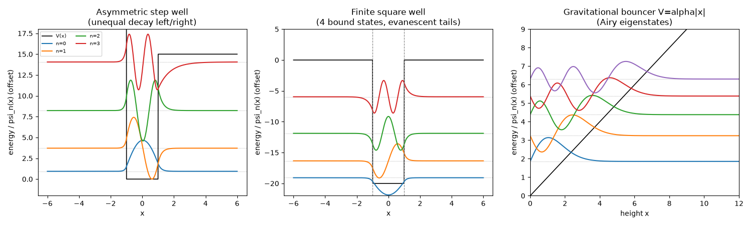
The bouncer’s numerically computed energies should match the exact Airy zeros closely.

print("Bouncer energies  (Numerov):", np.round(bouncer.energies, 4))
print("Bouncer energies  (Airy zeros, analytic):", np.round(analytic, 4))

Bouncer energies  (Numerov): [1.8558 3.2446 4.3817 5.3866 6.3053]
Bouncer energies  (Airy zeros, analytic): [1.8558 3.2446 4.3817 5.3866 6.3053]

A bound-state-count phase diagram over well depth and width

The finite square well above is one particular \((V_0,\text{width})\) pair; solving bound_states() on a coarse grid over both parameters (using a smaller grid/state count than above, just to keep the Numerov solve cheap at each point) maps out how many bound states the well supports, a genuine 2D map in place of a single well’s fixed-depth wavefunctions.

V0_grid = np.linspace(1.0, 40.0, 24)
width_grid = np.linspace(0.3, 4.0, 24)
n_bound_map = np.zeros((len(width_grid), len(V0_grid)))
for i, w in enumerate(width_grid):
    for j, v0 in enumerate(V0_grid):
        fsw_scan = FiniteSquareWell(V0=v0, width=w)
        eig = fsw_scan.bound_states(x_extent=max(6.0, 2 * w), n_points=300, n_states=20)
        n_bound_map[i, j] = int(np.sum(eig.energies < 0))

fig2, ax_map = plt.subplots(figsize=(7, 5))
im = ax_map.pcolormesh(V0_grid, width_grid, n_bound_map, shading="auto", cmap="viridis")
ax_map.plot([fsw.V0], [fsw.width], "o", color="red", ms=6, label="well used above")
ax_map.set_xlabel("Well depth V0")
ax_map.set_ylabel("Well width")
ax_map.set_title("Finite square well: number of bound states")
ax_map.legend(fontsize=8)
fig2.colorbar(im, ax=ax_map, label="# bound states", ticks=np.arange(0, n_bound_map.max() + 1))
fig2.tight_layout()

print(f"bound states at the well used above (V0={fsw.V0}, width={fsw.width}): {len(bound.energies)}")

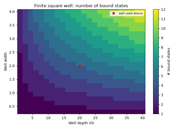
bound states at the well used above (V0=20.0, width=2.0): 4