Double-well tunneling

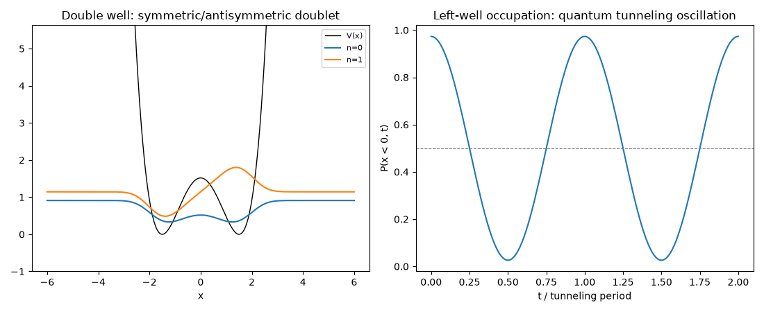
Builds the symmetric/antisymmetric doublet of \(V(x) = \lambda(x^2-a^2)^2\), then follows a wavepacket initially localized in the left well as it tunnels back and forth to the right well with period \(2\pi\hbar/\Delta E\).

import matplotlib.pyplot as plt
import numpy as np

from physicskit.quantum.chapters.potentials import DoubleWellSimulator
from physicskit.quantum.visualizers.wavefunctions import animate_density

dw = DoubleWellSimulator(lam=0.3, a=1.5)
result = dw.solve(n_states=4)

print(f"Doublet splitting  Delta E = {result.splitting:.6e}")
print(f"Tunneling period   T = {result.tunneling_period:.4f}")

Doublet splitting  Delta E = 2.328680e-01
Tunneling period   T = 26.9817

The doublet states and the resulting tunneling oscillation

fig, (ax1, ax2) = plt.subplots(1, 2, figsize=(11, 4.5))

# Potential + doublet wavefunctions
ax1.plot(dw.x, dw.V(dw.x), color="black", lw=1, label="V(x)")
for n in range(2):
    ax1.plot(dw.x, result.energies[n] + result.wavefunctions[n], label=f"n={n}")
ax1.set_ylim(-1, result.energies[3] + 2)
ax1.set_xlabel("x")
ax1.set_title("Double well: symmetric/antisymmetric doublet")
ax1.legend(fontsize=8)

# Tunneling oscillation: probability in the left well vs time
t = np.linspace(0, 2 * result.tunneling_period, 150)
P_left = dw.left_well_probability(result, t, side="left")
ax2.plot(t / result.tunneling_period, P_left)
ax2.set_xlabel("t / tunneling period")
ax2.set_ylabel("P(x < 0, t)")
ax2.set_title("Left-well occupation: quantum tunneling oscillation")
ax2.axhline(0.5, color="gray", ls="--", lw=0.8)

fig.tight_layout()

An animated, complex-valued version of the same oscillation

tunneling_wavefunction() gives the complex two-state wavefunction underlying the density-only tunneling_oscillation used above – an exact analytic evolution of the symmetric/antisymmetric doublet, distinct from the real FFT propagation used in A phase-colored tunneling animation – and animate_density() renders it frame by frame, phase-colored, as it tunnels back and forth.

t_anim = np.linspace(0, result.tunneling_period, 100)
frames = dw.tunneling_wavefunction(result, t_anim, side="left")
anim = animate_density(dw.x, frames, times=t_anim)
# anim.save("double_well_tunneling.gif", writer="pillow", fps=15)

The tunneling-splitting phase diagram over barrier height and separation

The single doublet splitting \(\Delta E\) used above is one point of \((\lambda, a)\); re-solving DoubleWellSimulator on a grid of both parameters shows \(\Delta E\) collapsing exponentially as the barrier separating the two wells grows taller (larger \(\lambda\)) or wider (larger \(a\)) – a genuine 2D map in place of the single well used for the wavepacket dynamics above.

lam_grid = np.linspace(0.1, 1.0, 12)
a_grid = np.linspace(1.0, 2.5, 12)
splitting_map = np.zeros((len(a_grid), len(lam_grid)))
for i, a_val in enumerate(a_grid):
    for j, lam_val in enumerate(lam_grid):
        dw_scan = DoubleWellSimulator(lam=lam_val, a=a_val, x_extent=max(6.0, a_val + 4.0), n_points=400)
        splitting_map[i, j] = dw_scan.solve(n_states=2).splitting

fig2, ax3 = plt.subplots(figsize=(7, 5))
im = ax3.pcolormesh(lam_grid, a_grid, np.log10(splitting_map), shading="auto", cmap="viridis")
ax3.plot([dw.lam], [dw.a], "o", color="red", ms=6, label="well used above")
ax3.set_xlabel(r"$\lambda$")
ax3.set_ylabel("a (half-separation)")
ax3.set_title(r"$\log_{10}(\Delta E)$: tunneling splitting collapses with barrier size")
ax3.legend(fontsize=8)
fig2.colorbar(im, ax=ax3, label=r"$\log_{10}(\Delta E)$")
fig2.tight_layout()

print(f"splitting at the (lambda, a) used above: {result.splitting:.4e}")
print(f"splitting range over the grid: [{splitting_map.min():.2e}, {splitting_map.max():.2e}]")

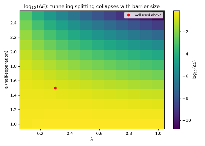
splitting at the (lambda, a) used above: 2.3287e-01
splitting range over the grid: [1.64e-11, 8.00e-01]