The Ramsauer-Townsend effect

Plots the exact transmission coefficient \(T(E)\) of a finite square well vs. incident energy. \(T(E)=1\) exactly whenever \(k_2 a\) is a multiple of \(\pi\) – the well becomes perfectly transparent, exactly as observed in low-energy electron scattering off noble-gas atoms.

import matplotlib.pyplot as plt
import numpy as np

from physicskit.quantum.chapters.potentials import FiniteSquareWell

V0, width = 10.0, 2.0
well = FiniteSquareWell(V0=V0, width=width)

E_values = np.linspace(0.05, 20, 3000)
T_values = well.transmission_spectrum(E_values)

# Resonances occur exactly where k2*a = n*pi, i.e. E_n = (n*pi/a)^2/2 - V0
resonance_n = np.arange(1, 6)
resonance_E = (resonance_n * np.pi / width) ** 2 / 2 - V0
resonance_E = resonance_E[resonance_E > 0]

The resonance curve, and the scattering potential for reference

fig, (ax1, ax2) = plt.subplots(1, 2, figsize=(11, 4.5))

ax1.plot(E_values, T_values)
for E_res in resonance_E:
    ax1.axvline(E_res, color="gray", ls=":", lw=0.8)
ax1.plot(resonance_E, np.ones_like(resonance_E), "o", color="red", label="T=1 resonances")
ax1.set_xlabel("Incident energy E")
ax1.set_ylabel("T(E)")
ax1.set_title(f"Ramsauer-Townsend resonances\n(well V0={V0}, width={width})")
ax1.legend(fontsize=8)

x = np.linspace(-3, 3, 500)
V = np.where(np.abs(x) <= width / 2, -V0, 0.0)
ax2.plot(x, V, color="black")
ax2.set_xlabel("x")
ax2.set_ylabel("V(x)")
ax2.set_title("The scattering potential")

fig.tight_layout()

for E_res in resonance_E:
    print(f"resonance at E={E_res:.4f}: T={well.scattering(E_res).T:.8f}")

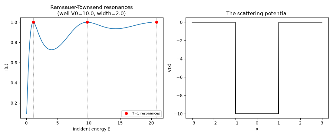
resonance at E=1.1033: T=1.00000000
resonance at E=9.7392: T=1.00000000
resonance at E=20.8425: T=1.00000000

An animated view: a wavepacket actually scattering off the well

The resonance curve above is the stationary scattering coefficient \(T(E)\). wavepacket_scattering() instead propagates a genuine moving Gaussian wavepacket at the well with the FFT split-operator method – the same shared method used for barrier tunneling in Real-time barrier tunneling, here with a positive well depth instead of a barrier – and animate_density() renders the reflected and transmitted pieces separating in real time.

from physicskit.quantum.visualizers.wavefunctions import animate_density  # noqa: E402

x_scatter, frames_scatter, times_scatter = well.wavepacket_scattering(
    x_extent=25.0,
    n_points=1024,
    x0=-10.0,
    sigma0=1.5,
    k0=None,
    dt=1e-3,
    n_steps=5000,
    save_every=100,
)
anim = animate_density(x_scatter, frames_scatter, times=times_scatter)
# anim.save("well_scattering.gif", writer="pillow", fps=15)

A 2D transmission map over energy and well width

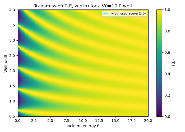
The resonance curve above fixes the well width and sweeps only the incident energy; transmission_spectrum() swept over both energy and width instead traces out the full family of \(T=1\) resonance lines (\(k_2 a = n\pi\)) at once, bending as the width changes – the perfectly-transparent Ramsauer-Townsend condition shown as a genuine 2D landscape rather than a single 1D scan.

E_map = np.linspace(0.05, 20.0, 200)
width_map = np.linspace(0.5, 4.0, 200)
T_map = np.zeros((len(width_map), len(E_map)))
for i, w in enumerate(width_map):
    well_w = FiniteSquareWell(V0=V0, width=w)
    T_map[i, :] = well_w.transmission_spectrum(E_map)

fig2, ax3 = plt.subplots(figsize=(7, 5))
im = ax3.pcolormesh(E_map, width_map, T_map, shading="auto", cmap="viridis", vmin=0, vmax=1)
ax3.axhline(width, color="cyan", ls="--", lw=1, label=f"width used above ({width})")
ax3.set_xlabel("Incident energy E")
ax3.set_ylabel("Well width")
ax3.set_title(f"Transmission T(E, width) for a V0={V0} well")
ax3.legend(fontsize=8)
fig2.colorbar(im, ax=ax3, label="T(E)")
fig2.tight_layout()