The Dirac equation and the fine structure of hydrogen

Dirac’s 1928 equation predicts the hydrogen levels exactly (apart from the tiny QED Lamb shift). Its energies, from dirac_hydrogen_energy(), depend on \(n\) and \(j\) only: each Bohr level \(n\) splits into \(n\) fine-structure sublevels, with \(2S_{1/2}\) and \(2P_{1/2}\) still degenerate. The splittings grow as \((Z\alpha)^4\), so they become large in heavy hydrogen-like ions.

import matplotlib.pyplot as plt
import numpy as np
from scipy.constants import fine_structure as alpha

from physicskit.quantum.chapters.relativistic import (
    dirac_hamiltonian,
    dirac_hydrogen_energy,
    fine_structure_expansion,
)

MC2_EV = 510998.95  # electron rest energy in eV
L_NAMES = "SPDFG"

Fine-structure levels of hydrogen

Binding energies relative to the Bohr energy \(-\alpha^2 mc^2/(2n^2)\), in \(\mu\mathrm{eV}\).

fig, ax = plt.subplots(figsize=(9, 5))
for n in (1, 2, 3, 4):
    bohr = -(alpha**2) / (2 * n**2)
    for j in np.arange(0.5, n, 1.0):
        shift = (dirac_hydrogen_energy(n, j) - 1 - bohr) * MC2_EV * 1e6
        ls = [ell for ell in (int(j - 0.5), int(j + 0.5)) if ell < n]
        label = ", ".join(f"{n}{L_NAMES[ell]}$_{{{int(2 * j)}/2}}$" for ell in ls)
        ax.hlines(shift, n - 0.3, n + 0.3, lw=2)
        ax.annotate(label, (n + 0.32, shift), va="center", fontsize=8)
ax.set_xticks([1, 2, 3, 4])
ax.set_xlabel("principal quantum number n")
ax.set_ylabel(r"$E_{nj} - E_n^{\rm Bohr}$ ($\mu$eV)")
ax.set_title("Dirac fine structure of hydrogen: levels depend on n and j only")
ax.set_xlim(0.5, 5.2)
fig.tight_layout()

split_2p = (dirac_hydrogen_energy(2, 1.5) - dirac_hydrogen_energy(2, 0.5)) * MC2_EV
print(f"2P3/2 - 2P1/2 splitting: {split_2p:.4e} eV = {split_2p / 4.135667696e-15 / 1e9:.2f} GHz")

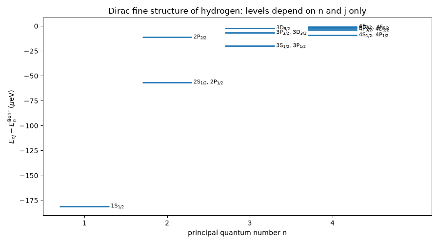
2P3/2 - 2P1/2 splitting: 4.5284e-05 eV = 10.95 GHz

Exact Dirac levels vs. the \((Z\alpha)^4\) expansion

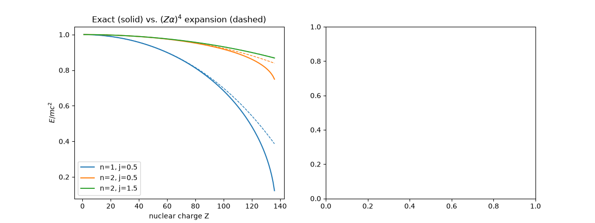
For light atoms the exact formula agrees with the fine-structure expansion of fine_structure_expansion(); for heavy ions the higher orders matter, and the ground state approaches \(E = mc^2\sqrt{1 - (Z\alpha)^2}\), which is only defined up to \(Z = 137\).

Z = np.arange(1, 137)
fig2, ax2 = plt.subplots(1, 2, figsize=(12, 4.5))
for n, j in ((1, 0.5), (2, 0.5), (2, 1.5)):
    exact = np.array([dirac_hydrogen_energy(n, j, z) for z in Z])
    ax2[0].plot(Z, exact, label=f"n={n}, j={j}")
    approx = np.array([1 + fine_structure_expansion(n, j, z) for z in Z])
    ax2[0].plot(Z, approx, "--", color=ax2[0].lines[-1].get_color(), lw=1)
ax2[0].set_xlabel("nuclear charge Z")
ax2[0].set_ylabel(r"$E / mc^2$")
ax2[0].set_title(r"Exact (solid) vs. $(Z\alpha)^4$ expansion (dashed)")
ax2[0].legend()

<matplotlib.legend.Legend object at 0x3706b71d0>

Positive and negative energies of the free Dirac equation

The free Dirac Hamiltonian \(\boldsymbol\alpha\cdot\mathbf p + \beta m\) has two doubly degenerate branches \(\pm\sqrt{p^2+m^2}\), separated by a gap of \(2mc^2\). Dirac interpreted the filled negative-energy “sea” as the origin of antiparticles.

p = np.linspace(-3, 3, 121)
bands = np.array([np.linalg.eigvalsh(dirac_hamiltonian([0, 0, pz])) for pz in p])
ax2[1].plot(p, bands, color="C0")
ax2[1].axhspan(-1, 1, color="0.9")
ax2[1].set_xlabel(r"$p_z / mc$")
ax2[1].set_ylabel(r"$E / mc^2$")
ax2[1].set_title(r"Free Dirac spectrum $E = \pm\sqrt{p^2 + m^2}$")
fig2.tight_layout()

Check

The 2P3/2 - 2P1/2 splitting is 10.95 GHz; at Z = 1 the alpha^4 expansion matches the exact Dirac energy to order alpha^6; the free Dirac bands are E = +-sqrt(p^2 + m^2), each doubly degenerate.

assert abs(split_2p / 4.135667696e-15 / 1e9 - 10.95) < 0.01
for n, j in ((1, 0.5), (2, 0.5), (2, 1.5)):
    assert abs(dirac_hydrogen_energy(n, j, 1) - 1 - fine_structure_expansion(n, j, 1)) < alpha**6
E_free = np.sqrt(1 + p**2)
np.testing.assert_allclose(bands, np.column_stack([-E_free, -E_free, E_free, E_free]), atol=1e-12)