The Born approximation: Rutherford scattering from quantum mechanics

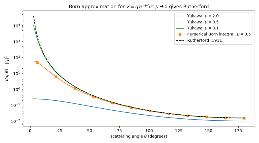
Max Born’s 1926 collision theory gives the scattering amplitude, to first order in the potential, as the Fourier transform of \(V(r)\) at the momentum transfer \(q = 2k\sin(\theta/2)\). For a screened Coulomb (Yukawa) potential \(V = g\,e^{-\mu r}/r\) it is \(f_B = -2mg/(\mu^2 + q^2)\). Removing the screening gives Rutherford’s classical 1911 cross section exactly. Here the numerical born_amplitude() is compared with the closed form and with rutherford_dsigma_domega().

import matplotlib.pyplot as plt
import numpy as np

from physicskit.particle.scattering import rutherford_dsigma_domega
from physicskit.quantum.chapters.scattering import born_amplitude, momentum_transfer, yukawa_born_amplitude

g, mass, k = 1.0, 1.0, 2.0  # coupling Z1 Z2 alpha, reduced mass, wavenumber
theta = np.linspace(0.05, np.pi, 300)
q = momentum_transfer(k, theta)
E_kin = k**2 / (2 * mass)

Screening length controls the forward peak

fig, ax = plt.subplots(figsize=(9, 5))
for mu in (2.0, 0.5, 0.1):
    ax.semilogy(np.degrees(theta), yukawa_born_amplitude(q, g, mu, mass) ** 2, label=rf"Yukawa, $\mu = {mu}$")
theta_num = np.linspace(0.1, np.pi, 12)
f_num = born_amplitude(lambda r: g * np.exp(-0.5 * r) / r, momentum_transfer(k, theta_num), mass)
ax.semilogy(np.degrees(theta_num), f_num**2, "o", color="C1", label=r"numerical Born integral, $\mu = 0.5$")
ax.semilogy(np.degrees(theta), rutherford_dsigma_domega(theta, 1, 1, E_kin, alpha=g), "k--", label="Rutherford (1911)")
ax.set_xlabel(r"scattering angle $\theta$ (degrees)")
ax.set_ylabel(r"$d\sigma/d\Omega = |f_B|^2$")
ax.set_title(r"Born approximation for $V = g\,e^{-\mu r}/r$: $\mu \to 0$ gives Rutherford")
ax.legend()
fig.tight_layout()

The Born amplitude is the Fourier transform of the potential

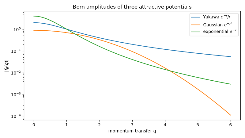
Different potentials with the same strength scatter differently because their Fourier transforms differ: a Gaussian well cuts off large momentum transfers exponentially, a Yukawa potential only as a power law.

q_grid = np.linspace(0, 6, 60)
potentials = {
    r"Yukawa $e^{-r}/r$": lambda r: -np.exp(-r) / r,
    r"Gaussian $e^{-r^2}$": lambda r: -np.exp(-(r**2)),
    r"exponential $e^{-r}$": lambda r: -np.exp(-r),
}
fig2, ax2 = plt.subplots(figsize=(8, 4.5))
for name, V in potentials.items():
    ax2.semilogy(q_grid, np.abs(born_amplitude(V, q_grid)), label=name)
ax2.set_xlabel("momentum transfer q")
ax2.set_ylabel(r"$|f_B(q)|$")
ax2.set_title("Born amplitudes of three attractive potentials")
ax2.legend()
fig2.tight_layout()

Check

The Yukawa Born amplitude is -2 m g / (q^2 + mu^2); the numerical Born integral reproduces it, and as mu -> 0 |f|^2 becomes Rutherford’s formula.

np.testing.assert_allclose(f_num, yukawa_born_amplitude(momentum_transfer(k, theta_num), g, 0.5, mass), rtol=1e-4)
np.testing.assert_allclose(yukawa_born_amplitude(q, g, 1e-8, mass) ** 2, rutherford_dsigma_domega(theta, 1, 1, E_kin, alpha=g), rtol=1e-8)