
Note
Go to the end to download the full example code.
Partial-wave analysis: phase shifts of the hard sphere and the square well#
Faxen and Holtsmark (1927) expanded scattering from a central potential
in angular-momentum partial waves. Each wave \(\ell\) is changed only
by a phase shift \(\delta_\ell\), and
\(\sigma = \frac{4\pi}{k^2}\sum_\ell(2\ell+1)\sin^2\delta_\ell\).
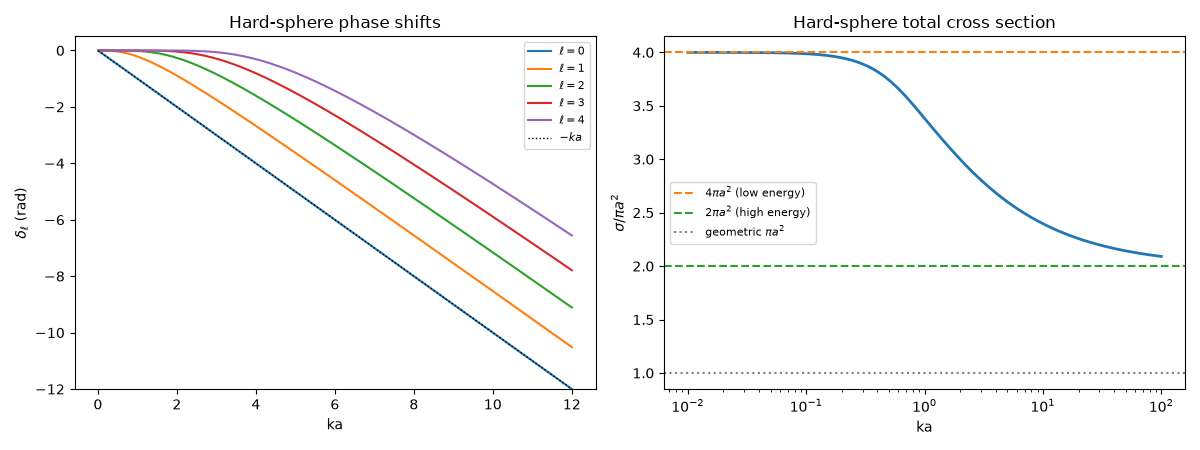
The hard sphere has exact phase shifts
(hard_sphere_phase_shifts());
its cross section goes from \(4\pi a^2\) at low energy to
\(2\pi a^2\) at high energy, twice the geometric area. For an
attractive square well,
partial_wave_phase_shifts()
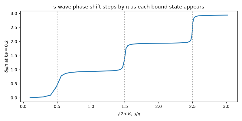
integrates Calogero’s variable-phase equation and finds the jumps of
\(\delta_0\) by \(\pi\) as bound states appear (Levinson’s
theorem).
import matplotlib.pyplot as plt
import numpy as np

from physicskit.quantum.chapters.scattering import (
    hard_sphere_phase_shifts,
    partial_wave_amplitude,
    partial_wave_cross_section,
    partial_wave_phase_shifts,
)

a = 1.0
Hard-sphere phase shifts and cross section#
Waves with \(\ell \gtrsim ka\) pass outside the sphere (classical impact parameter \(\ell/k > a\)) and are barely shifted.
ka = np.linspace(0.01, 12, 400)
deltas = np.array([hard_sphere_phase_shifts(k, a, 25) for k in ka])
fig, axes = plt.subplots(1, 2, figsize=(12, 4.5))
for ell in range(5):
    axes[0].plot(ka, np.unwrap(2 * deltas[:, ell]) / 2, label=rf"$\ell = {ell}$")
axes[0].plot(ka, -ka, "k:", lw=1, label=r"$-ka$")
axes[0].set_xlabel("ka")
axes[0].set_ylabel(r"$\delta_\ell$ (rad)")
axes[0].set_title("Hard-sphere phase shifts")
axes[0].legend(fontsize=8)
axes[0].set_ylim(-12, 0.5)

k_sig = np.logspace(-2, 2, 120)
sigma = [partial_wave_cross_section(k, hard_sphere_phase_shifts(k, a, int(k * a) + 30)) for k in k_sig]
axes[1].semilogx(k_sig, np.array(sigma) / (np.pi * a**2), lw=2)
axes[1].axhline(4, color="C1", ls="--", label=r"$4\pi a^2$ (low energy)")
axes[1].axhline(2, color="C2", ls="--", label=r"$2\pi a^2$ (high energy)")
axes[1].axhline(1, color="0.5", ls=":", label=r"geometric $\pi a^2$")
axes[1].set_xlabel("ka")
axes[1].set_ylabel(r"$\sigma / \pi a^2$")
axes[1].set_title("Hard-sphere total cross section")
axes[1].legend(fontsize=8)
fig.tight_layout()
Diffraction peak at high energy#
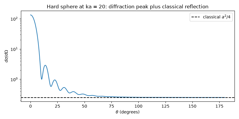
At \(ka = 20\) the angular distribution has a sharp forward (shadow) peak on top of the isotropic classical reflection.
k = 20.0
theta = np.linspace(0, np.pi, 800)
f = partial_wave_amplitude(theta, k, hard_sphere_phase_shifts(k, a, 60))
fig2, ax2 = plt.subplots(figsize=(8, 4))
ax2.semilogy(np.degrees(theta), np.abs(f) ** 2)
ax2.axhline(a**2 / 4, color="k", ls="--", label=r"classical $a^2/4$")
ax2.set_xlabel(r"$\theta$ (degrees)")
ax2.set_ylabel(r"$d\sigma/d\Omega$")
ax2.set_title(f"Hard sphere at ka = {k:.0f}: diffraction peak plus classical reflection")
ax2.legend()
fig2.tight_layout()
Square well: Levinson’s theorem#
Deepening an attractive well \(V = -V_0\,\Theta(a - r)\) binds a new s-wave state each time \(\sqrt{2mV_0}\,a\) passes an odd multiple of \(\pi/2\). At low energy (here \(ka = 0.2\)), \(\delta_0\) then rises steeply by \(\pi\).
k_low = 0.2
V0_grid = np.linspace(0.05, 45, 120)
d0 = [partial_wave_phase_shifts(lambda r, V0=V0: np.where(r < a, -V0, 0.0), k_low, 0, r_max=a + 0.2, breakpoints=[a], rtol=1e-7)[0] for V0 in V0_grid]
fig3, ax3 = plt.subplots(figsize=(8, 4))
ax3.plot(np.sqrt(2 * V0_grid) * a / np.pi, np.array(d0) / np.pi, lw=2)
for n in range(1, 4):
    ax3.axvline(n - 0.5, color="0.6", ls=":")
ax3.set_xlabel(r"$\sqrt{2mV_0}\,a/\pi$")
ax3.set_ylabel(r"$\delta_0/\pi$ at $ka = 0.2$")
ax3.set_title("s-wave phase shift steps by π as each bound state appears")
fig3.tight_layout()
Check#
Hard sphere: delta_0 = -ka (mod pi); sigma -> 4 pi a^2 at low energy (four times the geometric cross section) and -> 2 pi a^2 at high energy (the shadow doubles it). Square well: Levinson’s theorem, delta_0 -> N pi with N = 3 bound s-states for sqrt(2 V0) a / pi = 3.02.
Total running time of the script: (0 minutes 4.872 seconds)