De Broglie’s matter wave

Builds a free Gaussian wavepacket carrying de Broglie’s traveling-wave factor \(e^{ik_0 x}\) via free_gaussian_wavepacket(), and verifies that its momentum-space density peaks exactly at \(p_0=\hbar k_0\), so the associated wavelength is de Broglie’s \(\lambda = h/p\).

import matplotlib.pyplot as plt
import numpy as np

from physicskit.quantum.chapters.wave_packets import free_gaussian_wavepacket
from physicskit.quantum.utils.measure import momentum_density
from physicskit.quantum.visualizers.phase_space import WignerVisualizer

x0, sigma0, k0 = 0.0, 2.0, 3.0
x = np.linspace(-20, 20, 4000)
psi0 = free_gaussian_wavepacket(x, x0=x0, sigma0=sigma0, k0=k0)

p, psi_p = momentum_density(x, psi0)
p_peak = p[np.argmax(np.abs(psi_p) ** 2)]

Real/imaginary parts reveal the de Broglie phase \(e^{ik_0 x}\), and the momentum-space density peaks at \(p_0=\hbar k_0\) ————————————————————————–

fig, axes = plt.subplots(1, 2, figsize=(11, 4.5))

axes[0].plot(x, np.abs(psi0) ** 2, color="black", lw=1.5, label=r"$|\psi(x)|^2$ (envelope)")
axes[0].plot(x, np.real(psi0), lw=1, alpha=0.8, label=r"Re $\psi(x)$")
axes[0].plot(x, np.imag(psi0), lw=1, alpha=0.8, label=r"Im $\psi(x)$")
axes[0].set_xlim(-8, 8)
axes[0].set_xlabel("x")
axes[0].set_title(r"Free Gaussian wavepacket carrying $e^{ik_0 x}$")
axes[0].legend(fontsize=8)

axes[1].plot(p, np.abs(psi_p) ** 2)
axes[1].axvline(k0, color="gray", ls="--", label=r"$p_0=\hbar k_0$" f"={k0}")
axes[1].set_xlim(k0 - 3, k0 + 3)
axes[1].set_xlabel("p")
axes[1].set_title("Momentum-space density")
axes[1].legend(fontsize=8)

fig.tight_layout()

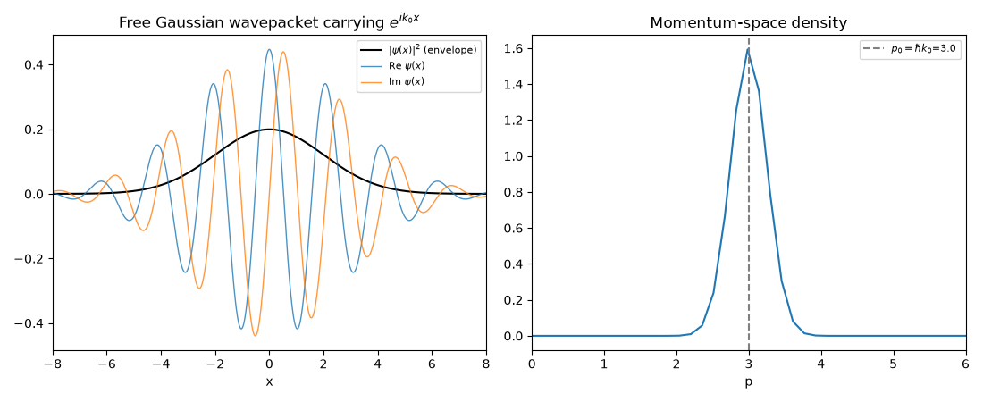
de Broglie’s relation \(\lambda = h/p = 2\pi/k_0\) (with \(\hbar=1\)) checked against the wavelength read directly off the phase \(e^{ik_0 x}\).

lambda_de_broglie = 2 * np.pi / p_peak
print(f"momentum-space peak: p_peak={p_peak:.4f}  (expected p_0=hbar*k_0={k0})")
print(f"de Broglie wavelength lambda=2*pi/p_peak={lambda_de_broglie:.4f}  (expected 2*pi/k0={2 * np.pi / k0:.4f})")

momentum-space peak: p_peak=2.9838  (expected p_0=hbar*k_0=3.0)
de Broglie wavelength lambda=2*pi/p_peak=2.1058  (expected 2*pi/k0=2.0944)

The same wave in phase space: a single Wigner-function blob

The position- and momentum-space pictures above are two 1D projections of one underlying phase-space object; WignerVisualizer combines them into a single \(W(x,p)\) quasi-probability distribution – for a Gaussian wavepacket it is a positive Gaussian blob centered exactly at \((x_0, p_0=\hbar k_0)\), directly showing de Broglie’s wave simultaneously localized (loosely) in both position and momentum.

wv = WignerVisualizer(n_p=200)
xg, pg, W = wv.compute(x, psi0, p_max=k0 + 3)

fig2, ax_w = plt.subplots(figsize=(6.5, 5))
wv.plot_contour(xg, pg, W, ax=ax_w)
ax_w.axvline(x0, color="cyan", ls="--", lw=0.8)
ax_w.axhline(k0, color="cyan", ls="--", lw=0.8, label=f"(x0, hbar*k0)=({x0}, {k0})")
ax_w.set_xlim(x0 - 8, x0 + 8)
ax_w.set_title("Wigner phase-space distribution\nof the free Gaussian wavepacket")
ax_w.legend(fontsize=8)
fig2.tight_layout()

print(f"Wigner peak location (x,p) index vs. expected ({x0}, {k0}): min W={W.min():.2e} (Gaussian states have W>=0)")

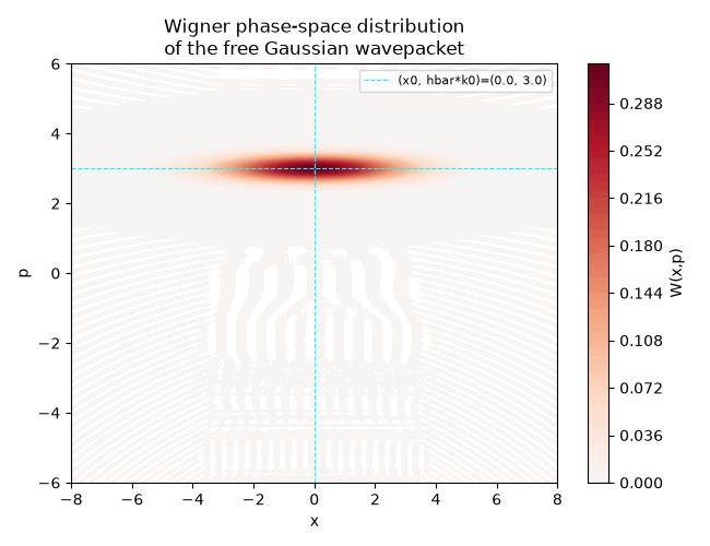
Wigner peak location (x,p) index vs. expected (0.0, 3.0): min W=-4.35e-13 (Gaussian states have W>=0)