Ehrenfest’s theorem in an anharmonic well

Ehrenfest’s theorem states that quantum expectation values obey the classical equations of motion exactly:

\[\frac{d\langle x\rangle}{dt} = \frac{\langle p\rangle}{m}, \qquad \frac{d\langle p\rangle}{dt} = -\left\langle \frac{dV}{dx}\right\rangle.\]

This holds for any potential, not just harmonic ones – unlike the naive classical trajectory, which would use \(-dV/dx(\langle x\rangle)\) and only coincides with \(-\langle dV/dx\rangle\) when \(V\) is quadratic. Verified here for the quartic well \(V(x) = 0.25 x^4\) by comparing both sides of each equation, computed independently from a real wavepacket propagation.

import matplotlib.pyplot as plt
import numpy as np

from physicskit.quantum.core.solvers import SplitOperatorSolver1D
from physicskit.quantum.utils.measure import ExpectationMonitor, expectation_value
from physicskit.quantum.visualizers.phase_space import WignerVisualizer

x = np.linspace(-8, 8, 2048)


def V(x):
    return 0.25 * x**4


def dV_dx(x):
    return x**3


solver = SplitOperatorSolver1D(x, V, dt=2e-4)
psi0 = np.exp(-((x - 1.5) ** 2) / (2 * 0.5**2)) * np.exp(1j * 0.5 * x)
psi0 = psi0.astype(complex)
psi0 /= np.sqrt(solver.norm(psi0))

n_steps = 6000
save_every = 10
frames, times = solver.propagate(psi0, n_steps, save_every=save_every)

monitor = ExpectationMonitor(x)
monitor.record_all(times, frames)
h = monitor.as_arrays()

# <dV/dx>(t), computed directly from each snapshot (the RHS of Ehrenfest's
# second equation) -- independent of the <x>(t), <p>(t) already recorded.
dV_expectation = np.array([np.real(expectation_value(lambda xx, psi: dV_dx(xx) * psi, x, psi)) for psi in frames])

# Numerical time derivatives of the recorded <x>(t), <p>(t)
dxdt = np.gradient(h["x"], h["t"])
dpdt = np.gradient(h["p"], h["t"])

Both sides of each Ehrenfest identity, computed independently

fig, axes = plt.subplots(1, 3, figsize=(15, 4.5))

axes[0].plot(x, V(x), color="black", lw=1)
axes[0].plot(h["x"], V(h["x"]), color="red", lw=1, alpha=0.5, label="<x>(t) trajectory (on V)")
axes[0].set_xlim(-6, 6)
axes[0].set_ylim(-2, 60)
axes[0].set_xlabel("x")
axes[0].set_title(r"Quartic well $V(x)=\frac{1}{4}x^4$")
axes[0].legend(fontsize=8)

axes[1].plot(h["t"], dxdt, label=r"$d\langle x\rangle/dt$ (numeric)")
axes[1].plot(h["t"], h["p"], "--", label=r"$\langle p\rangle/m$")
axes[1].set_xlabel("t")
axes[1].set_title(r"Ehrenfest I: $d\langle x\rangle/dt = \langle p\rangle/m$")
axes[1].legend(fontsize=8)

axes[2].plot(h["t"], dpdt, label=r"$d\langle p\rangle/dt$ (numeric)")
axes[2].plot(h["t"], -dV_expectation, "--", label=r"$-\langle dV/dx\rangle$")
axes[2].set_xlabel("t")
axes[2].set_title(r"Ehrenfest II: $d\langle p\rangle/dt = -\langle dV/dx\rangle$")
axes[2].legend(fontsize=8)

fig.tight_layout()

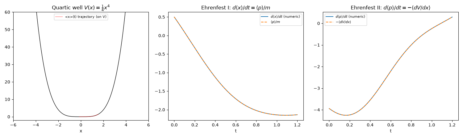
Both identities hold to within the finite-difference time-derivative resolution.

max_err_1 = np.max(np.abs(dxdt[2:-2] - h["p"][2:-2]))
max_err_2 = np.max(np.abs(dpdt[2:-2] - (-dV_expectation[2:-2])))
print(f"max |d<x>/dt - <p>|   = {max_err_1:.2e}")
print(f"max |d<p>/dt + <dV/dx>| = {max_err_2:.2e}")
print(f"norm conservation check: {solver.norm(frames[-1]):.8f}")

max |d<x>/dt - <p>|   = 4.64e-06
max |d<p>/dt + <dV/dx>| = 1.78e-05
norm conservation check: 1.00000000

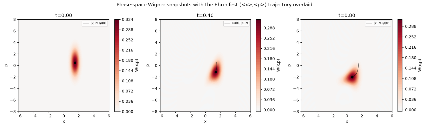
The state in phase space: Wigner-function snapshots with the Ehrenfest trajectory overlaid ————————————————————————–

Position space and the two expectation-value identities above never show the full quantum state at once; WignerVisualizer applied to the same propagated frames used for monitor shows the state’s phase-space blob directly, with the classical-like \((\langle x\rangle(t),\langle p\rangle(t))\) trajectory traced by Ehrenfest’s theorem drawn on top – in this anharmonic well the blob visibly shears and distorts as it evolves, unlike the rigid rotation a harmonic-oscillator coherent state’s Wigner blob would undergo.

wv = WignerVisualizer(n_p=150)
snap_idx = [0, len(frames) // 3, 2 * len(frames) // 3]

fig2, axes2 = plt.subplots(1, len(snap_idx), figsize=(15, 4.5))
for ax, i in zip(axes2, snap_idx):
    xg, pg, W = wv.compute(x, frames[i], p_max=8.0)
    wv.plot_contour(xg, pg, W, ax=ax)
    ax.plot(h["x"][: i + 1], h["p"][: i + 1], color="black", lw=1, alpha=0.7, label=r"$\langle x\rangle(t),\langle p\rangle(t)$")
    ax.plot(h["x"][i], h["p"][i], "o", color="black", ms=5)
    ax.set_xlim(-6, 6)
    ax.set_title(f"t={h['t'][i]:.2f}")
    ax.legend(fontsize=7, loc="upper right")
fig2.suptitle("Phase-space Wigner snapshots with the Ehrenfest (<x>,<p>) trajectory overlaid")
fig2.tight_layout()