Einstein predicts gravitational waves: polarizations and the quadrupole formula

Linearizing his field equations in 1916, and correcting a factor of two in 1918, Einstein found that ripples of spacetime travel at the speed of light with two transverse polarizations, \(+\) and \(\times\), and that a system radiates them in proportion to the third time derivative of its mass quadrupole moment. For two masses on a circular orbit of separation \(a\) the radiated power is

\[P = \frac{32}{5}\,\frac{G^4}{c^5}\,\frac{(m_1m_2)^2(m_1+m_2)}{a^5}.\]

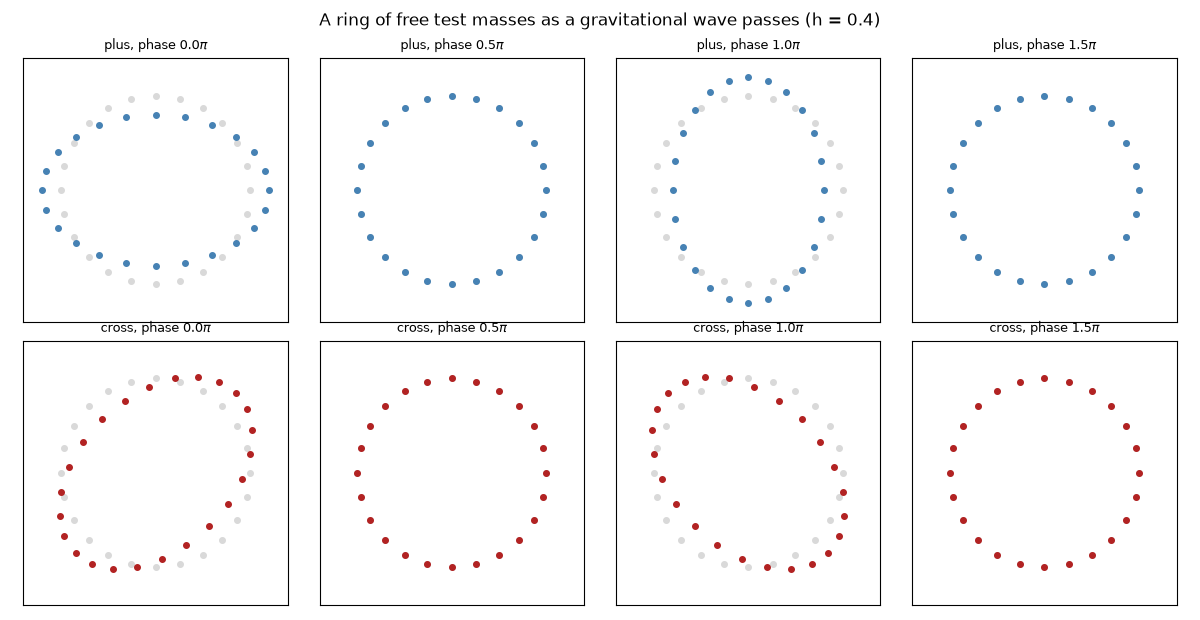
This example shows what each polarization does to a ring of free test masses, evaluates the quadrupole power for the Earth-Sun system and for a compact binary, and follows the leading-order chirp \(f(t)\propto(t_c-t)^{-3/8}\) that the energy loss drives, using inspiral_frequency() and inspiral_strain().

import matplotlib.pyplot as plt
import numpy as np

from physicskit.relativity.chapters.gw_merger import BinaryMerger
from physicskit.relativity.utils import constants as const

G, c, MSUN = const.G_SI, const.C_SI, const.SOLAR_MASS_KG

The two polarizations

A wave travelling along z with strain \(h\) moves a free particle at \((x, y)\) by \(\delta x = \tfrac12(h_+x + h_\times y)\), \(\delta y = \tfrac12(h_\times x - h_+y)\). The \(+\) mode stretches along x while squeezing along y, then the reverse; the \(\times\) mode does the same along the diagonals.

phi = np.linspace(0, 2 * np.pi, 24, endpoint=False)
x0, y0 = np.cos(phi), np.sin(phi)
h = 0.4  # hugely exaggerated for visibility
phases = np.linspace(0, 2 * np.pi, 5)[:-1]
fig1, axes = plt.subplots(2, 4, figsize=(12, 6.2))
for row, (name, hp_amp, hx_amp) in enumerate([("plus", h, 0.0), ("cross", 0.0, h)]):
    for ax, ph in zip(axes[row], phases):
        hp, hx = hp_amp * np.cos(ph), hx_amp * np.cos(ph)
        x = x0 + 0.5 * (hp * x0 + hx * y0)
        y = y0 + 0.5 * (hx * x0 - hp * y0)
        ax.plot(x0, y0, "o", color="0.85", ms=4)
        ax.plot(x, y, "o", color="steelblue" if row == 0 else "firebrick", ms=4)
        ax.set_xlim(-1.4, 1.4)
        ax.set_ylim(-1.4, 1.4)
        ax.set_aspect("equal")
        ax.set_xticks([])
        ax.set_yticks([])
        ax.set_title(f"{name}, phase {ph / np.pi:.1f}$\\pi$", fontsize=9)
fig1.suptitle("A ring of free test masses as a gravitational wave passes (h = 0.4)")
fig1.tight_layout()

The quadrupole formula

Einstein himself judged the effect hopelessly small. The Earth-Sun system radiates about 200 W. Two neutron stars a few hundred kilometres apart radiate more than the Sun’s light output.

def quadrupole_power(m1, m2, a):
    return 32 / 5 * G**4 / c**5 * (m1 * m2) ** 2 * (m1 + m2) / a**5


P_earth = quadrupole_power(MSUN, 5.972e24, 1.496e11)
P_ns = quadrupole_power(1.4 * MSUN, 1.4 * MSUN, 300e3)
print(f"Earth-Sun:                  P = {P_earth:.0f} W")
print(f"two 1.4 Msun neutron stars 300 km apart: P = {P_ns:.2e} W  ({P_ns / 3.828e26:.1e} solar luminosities)")

Earth-Sun:                  P = 196 W
two 1.4 Msun neutron stars 300 km apart: P = 7.22e+42 W  (1.9e+16 solar luminosities)

Energy loss drives a chirp

Losing energy shrinks the orbit, which speeds it up and makes it radiate harder. The gravitational-wave frequency (twice the orbital frequency) runs away as \((t_c-t)^{-3/8}\), with a rate set by the chirp mass \(\mathcal M=(m_1m_2)^{3/5}/(m_1+m_2)^{1/5}\) alone.

binary = BinaryMerger(const.solar_masses_to_geometrized(1.4), const.solar_masses_to_geometrized(1.4), distance=40e6 * const.PARSEC_M)
tau_s = np.geomspace(1e-3, 100.0, 300)  # seconds before coalescence
f = binary.inspiral_frequency(-const.seconds_to_geometrized(tau_s), 0.0) * c
slope = np.polyfit(np.log(tau_s), np.log(f), 1)[0]
print(f"\nd ln f / d ln(t_c - t) = {slope:.4f}  (Einstein's quadrupole formula: -3/8 = -0.375)")
print(f"f at 100 s before merger: {f[-1]:.1f} Hz; at 1 ms: {f[0]:.0f} Hz")

t_s = np.linspace(-2.0, -0.002, 20000)
hp, _ = binary.inspiral_strain(const.seconds_to_geometrized(t_s), 0.0)

fig2, (ax1, ax2) = plt.subplots(1, 2, figsize=(11, 3.8))
ax1.loglog(tau_s, f, color="steelblue")
ax1.set_xlabel("time before coalescence [s]")
ax1.set_ylabel("GW frequency [Hz]")
ax1.set_title(r"$f \propto (t_c - t)^{-3/8}$")
ax2.plot(t_s, hp, color="firebrick", lw=0.5)
ax2.set_xlabel("time [s]")
ax2.set_ylabel(r"$h_+$ at 40 Mpc")
ax2.set_title("Neutron-star inspiral: the last two seconds")
fig2.tight_layout()

plt.show()

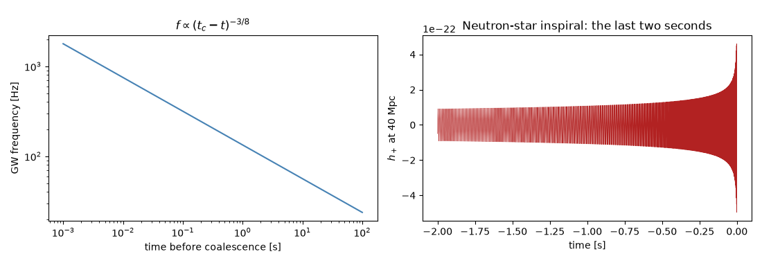
d ln f / d ln(t_c - t) = -0.3750  (Einstein's quadrupole formula: -3/8 = -0.375)
f at 100 s before merger: 23.7 Hz; at 1 ms: 1780 Hz

Check

The Earth-Sun system radiates ~200 W; the inspiral frequency follows f ~ (t_c - t)^(-3/8).

assert 150 < P_earth < 250
assert abs(slope + 3 / 8) < 1e-3