Numerical relativity solves the binary black hole merger

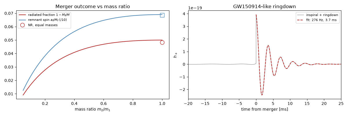
For decades after the ADM equations, nobody could evolve two black holes through merger on a computer: simulations crashed long before the holes met. In 2005 Pretorius, and weeks later the Campanelli and Baker groups with “moving punctures”, succeeded. The simulations answered questions no approximation could. How much of the binary’s mass is radiated in the final orbits and merger? About 5% for equal masses. How fast does the single remnant spin? \(a_f/M_f\approx0.69\). And the remnant then rings down at the quasinormal-mode frequency of that Kerr black hole.

This example uses remnant_estimate(), which is anchored to those numerical-relativity results, to follow the remnant’s mass and spin across mass ratios. It computes the ringdown frequency and damping time with qnm_frequency_damping(), then recovers both by fitting the post-merger part of full_waveform(), the way remnant properties are read off a measured signal.

import matplotlib.pyplot as plt
import numpy as np
from scipy.optimize import curve_fit

from physicskit.relativity.chapters.gw_merger import BinaryMerger
from physicskit.relativity.utils import constants as const

What the simulations measured

For non-spinning equal-mass black holes, high-accuracy simulations (Scheel et al. 2009) give \(M_f = 0.95162\,M\) and \(a_f/M_f = 0.68646\). The remnant is a rapidly spinning Kerr hole, and about 4.8% of the rest mass leaves as gravitational waves.

M_sun_geom = const.solar_masses_to_geometrized(1.0)
q_values = np.linspace(0.05, 1.0, 40)  # mass ratio m2/m1
M_f_frac, spin = [], []
for q in q_values:
    bm = BinaryMerger(M_sun_geom * 30, M_sun_geom * 30 * q, distance=1e25)
    M_f, a_f = bm.remnant_estimate()
    M_f_frac.append(M_f / bm.total_mass)
    spin.append(a_f / M_f)
M_f_frac, spin = np.array(M_f_frac), np.array(spin)
print(f"equal masses: M_f/M = {M_f_frac[-1]:.4f} (NR 0.9516), a_f/M_f = {spin[-1]:.3f} (NR 0.686)")

equal masses: M_f/M = 0.9500 (NR 0.9516), a_f/M_f = 0.690 (NR 0.686)

GW150914’s remnant and ringdown

36 and 29 solar masses merge into a hole of about 62 solar masses spinning at about 0.69 of its maximum. Its dominant quasinormal mode rings at a few hundred hertz and dies away in a few milliseconds.

m1, m2 = const.solar_masses_to_geometrized(36.0), const.solar_masses_to_geometrized(29.0)
gw150914 = BinaryMerger(m1, m2, distance=410e6 * const.PARSEC_M)
M_f, a_f = gw150914.remnant_estimate()
f_qnm, tau = gw150914.qnm_frequency_damping()
f_Hz = f_qnm * const.C_SI
tau_ms = const.geometrized_to_seconds(tau) * 1e3
E_rad = const.geometrized_to_solar_masses(gw150914.total_mass - M_f)
print(f"\nGW150914 remnant: {const.geometrized_to_solar_masses(M_f):.1f} Msun, spin {a_f / M_f:.2f}; radiated {E_rad:.1f} Msun c^2")
print(f"ringdown: f_QNM = {f_Hz:.0f} Hz, damping time {tau_ms:.2f} ms")

GW150914 remnant: 61.8 Msun, spin 0.68; radiated 3.2 Msun c^2
ringdown: f_QNM = 276 Hz, damping time 3.71 ms

Reading the remnant off the ringdown

Fit a damped sinusoid to the strain after merger. The fitted frequency and damping time identify the remnant’s mass and spin: this is the black-hole spectroscopy that numerical-relativity waveforms made possible.

t_s = np.linspace(-0.05, 0.03, 20000)
hp, _ = gw150914.full_waveform(const.seconds_to_geometrized(t_s), 0.0)
post = t_s >= 0


def damped(t, A, f, tau_d, phase):
    return A * np.exp(-t / tau_d) * np.cos(2 * np.pi * f * t + phase)


A0 = np.abs(hp[post]).max()
popt, _ = curve_fit(damped, t_s[post], hp[post], p0=[A0, 250.0, 0.004, 0.0])
print(f"fitted ringdown: f = {popt[1]:.1f} Hz, tau = {popt[2] * 1e3:.2f} ms  (input {f_Hz:.1f} Hz, {tau_ms:.2f} ms)")

fig, (ax1, ax2) = plt.subplots(1, 2, figsize=(12, 4))
ax1.plot(q_values, 1 - M_f_frac, color="firebrick", label=r"radiated fraction $1 - M_f/M$")
ax1.plot(q_values, spin / 10, color="steelblue", label=r"remnant spin $a_f/M_f$ (/10)")
ax1.plot([1.0], [1 - 0.95162], "o", color="firebrick", mfc="none", ms=10, label="NR, equal masses")
ax1.plot([1.0], [0.68646 / 10], "s", color="steelblue", mfc="none", ms=10)
ax1.set_xlabel("mass ratio $m_2/m_1$")
ax1.set_title("Merger outcome vs mass ratio")
ax1.legend(fontsize=8)
ax2.plot(t_s * 1e3, hp, color="0.5", lw=0.8, label="inspiral + ringdown")
ax2.plot(t_s[post] * 1e3, damped(t_s[post], *popt), "--", color="firebrick", label=f"fit: {popt[1]:.0f} Hz, {popt[2] * 1e3:.1f} ms")
ax2.set_xlim(-20, 25)
ax2.set_xlabel("time from merger [ms]")
ax2.set_ylabel(r"$h_+$")
ax2.set_title("GW150914-like ringdown")
ax2.legend(fontsize=8)
fig.tight_layout()

plt.show()

/Users/cpoli/Code/physicskit/examples/relativity/gravitational_waves/plot_numerical_relativity_merger.py:85: OptimizeWarning: Covariance of the parameters could not be estimated
  popt, _ = curve_fit(damped, t_s[post], hp[post], p0=[A0, 250.0, 0.004, 0.0])
fitted ringdown: f = 275.8 Hz, tau = 3.71 ms  (input 275.8 Hz, 3.71 ms)

Check

Equal-mass remnant: M_f / M = 0.9516, a_f / M_f = 0.686 (numerical relativity); the ringdown fit recovers the quasinormal mode.

assert abs(M_f_frac[-1] - 0.9516) < 0.003 and abs(spin[-1] - 0.686) < 0.01
assert abs(popt[1] / f_Hz - 1) < 0.01 and abs(popt[2] * 1e3 / tau_ms - 1) < 0.01