Spaghettification: tidal forces near a black hole

An object falling toward a black hole isn’t crushed from all sides – it is stretched along the radial direction (the near side is pulled harder than the far side) and squeezed along the two transverse directions. In the local orthonormal frame of a freely-falling observer, two points separated by a small proper length \(\ell\) experience a relative (geodesic deviation) acceleration

\[a_{\text{radial}} = \frac{2M}{r^3}\,\ell, \qquad a_{\text{transverse}} = -\frac{M}{r^3}\,\ell\]

both growing as \(1/r^3\) and formally diverging at the singularity. This is tidal gravity: the same effect that raises ocean tides on Earth, scaled up by many orders of magnitude near a stellar-mass black hole. This example plots how quickly these accelerations grow as an infalling astronaut (proper separation \(\ell = 1.8\) m, head to toe) approaches the horizon, and compares the tidal stretch actually felt at the horizon of a 10-solar-mass black hole against a supermassive one like Sgr A*.

import matplotlib.pyplot as plt
import numpy as np

import physicskit.relativity.utils.constants as const
from physicskit.relativity.chapters.schwarzschild import SchwarzschildBlackHole

Tidal acceleration grows sharply approaching the horizon

bh = SchwarzschildBlackHole(M=1.0)
r = np.linspace(bh.horizon_radius * 1.01, 20.0, 300)
radial, transverse = bh.tidal_acceleration(r, proper_separation=1.0)

fig, ax = plt.subplots(figsize=(7, 4.5))
ax.plot(r, radial, label="radial (stretching)")
ax.plot(r, -transverse, label="transverse (compression)", linestyle="--")
ax.axvline(bh.horizon_radius, color="k", linestyle=":", linewidth=1, label="horizon")
ax.set_yscale("log")
ax.set_xlabel("r [M]")
ax.set_ylabel("tidal acceleration per unit length [1/M$^2$]")
ax.set_title("Tidal (geodesic deviation) acceleration vs. radius")
ax.legend()
plt.tight_layout()

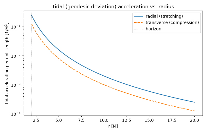
For a stellar-mass black hole, spaghettification happens well outside the horizon; for a supermassive black hole, an astronaut could cross the horizon completely unharmed ——————————————————————————–

human_height_m = 1.8
for mass_solar, label in [(10.0, "10 solar-mass BH"), (1.0e6, "10^6 solar-mass BH (Sgr A*-like)")]:
    M_geom = const.solar_masses_to_geometrized(mass_solar)
    bh_m = SchwarzschildBlackHole(M=M_geom)
    radial_at_horizon, _ = bh_m.tidal_acceleration(bh_m.horizon_radius, proper_separation=human_height_m)
    tidal_g = radial_at_horizon * const.C_SI**2 / 9.81  # convert (1/s^2)*m to units of g
    print(f"{label}: tidal stretch at the horizon = {tidal_g:.3e} g")

10 solar-mass BH: tidal stretch at the horizon = 1.891e+07 g
10^6 solar-mass BH (Sgr A*-like): tidal stretch at the horizon = 1.891e-03 g

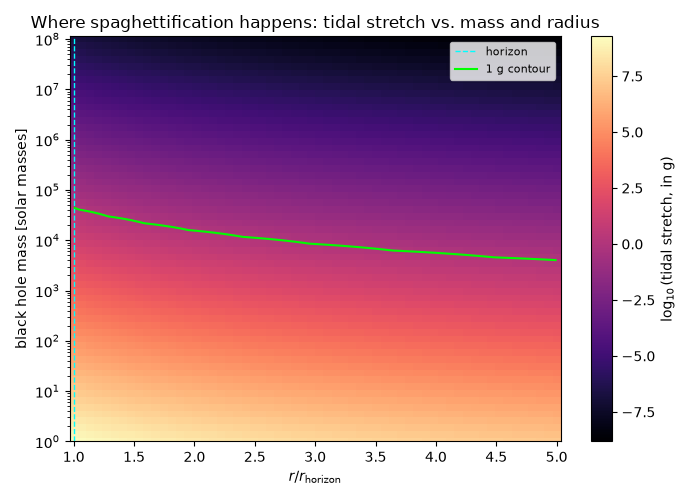
Where spaghettification happens, as a continuous function of mass and radius

The two-point comparison above is one slice of a much bigger picture: tidal_acceleration() scales as \(1/M^2\) at fixed \(r/r_{\text{horizon}}\) (since \(r \propto M\)), so a continuous map over both mass and radius shows exactly which black holes spaghettify an infalling astronaut well outside the horizon, and which – like Sgr A* – let one cross completely unharmed.

masses_solar = np.logspace(0.0, 8.0, 60)
r_over_horizon = np.linspace(1.0, 5.0, 60)
tidal_g_map = np.zeros((len(masses_solar), len(r_over_horizon)))
for i, mass_solar in enumerate(masses_solar):
    bh_m = SchwarzschildBlackHole(M=const.solar_masses_to_geometrized(mass_solar))
    r_vals = r_over_horizon * bh_m.horizon_radius
    radial, _ = bh_m.tidal_acceleration(r_vals, proper_separation=human_height_m)
    tidal_g_map[i] = radial * const.C_SI**2 / 9.81

fig, ax = plt.subplots(figsize=(7, 5))
im = ax.pcolormesh(r_over_horizon, masses_solar, np.log10(tidal_g_map), shading="auto", cmap="magma")
ax.set_yscale("log")
plt.colorbar(im, ax=ax, label=r"$\log_{10}$(tidal stretch, in g)")
ax.axvline(1.0, color="cyan", linestyle="--", linewidth=1, label="horizon")
ax.contour(r_over_horizon, masses_solar, tidal_g_map, levels=[1.0], colors="lime", linewidths=1.5)
ax.plot([], [], color="lime", label="1 g contour")
ax.set_xlabel(r"$r / r_{\text{horizon}}$")
ax.set_ylabel("black hole mass [solar masses]")
ax.set_title("Where spaghettification happens: tidal stretch vs. mass and radius")
ax.legend(fontsize=8)
plt.tight_layout()
plt.show()