Penrose’s singularity theorems: finite proper time, divergent coordinate time

Long before Penrose’s 1965 proof that trapped surfaces force geodesic incompleteness regardless of symmetry, a simpler, coordinate-dependent puzzle already hinted that something was wrong with treating Schwarzschild coordinate time \(t\) as a universal clock: a particle dropped from rest at radius \(R\) reaches the true singularity in finite proper time,

\[\tau_{r=0} = \frac{\pi}{2}\sqrt{\frac{R^3}{2M}},\]

even though the same infall, described in Schwarzschild \(t\), takes forever – \(t\to\infty\) as the particle approaches the horizon. This example integrates exactly that radial plunge with eccentric_orbit_initial_state() and integrate_geodesic(), and shows both halves directly: proper time accumulates normally all the way to the horizon, while \(dt/d\tau\) grows without bound over the same interval. Schwarzschild coordinates become singular exactly at the horizon, so the integrator – built on this same coordinate time – cannot be pushed any further inward at all; reaching the true singularity needs the closed-form \(\tau_{r=0}\) above, evaluated directly rather than integrated numerically.

import matplotlib.pyplot as plt
import numpy as np

from physicskit.relativity.chapters.schwarzschild import SchwarzschildBlackHole

A radial plunge from rest

eccentricity_boost=1.0 removes all tangential velocity, giving a purely radial infall starting from rest at r0.

M = 1.0
bh = SchwarzschildBlackHole(M=M)
R0 = 10.0

y0 = bh.eccentric_orbit_initial_state(R0, eccentricity_boost=1.0)
print(f"initial 4-velocity (t,r,theta,phi,u^t,u^r,u^theta,u^phi): {np.round(y0, 6)}")
print("(u^r = u^phi = 0: purely radial, released from rest)")

dtau = 0.001
trajectory = bh.integrate_geodesic(y0, dtau, n_steps=200_000)
r = trajectory["r"]
t = trajectory["t"]
tau = np.arange(len(r)) * dtau

print(f"\nhorizon radius: r_s = {bh.horizon_radius}")
print(f"integration halts at r = {r[-1]:.6f} (just outside the horizon -- Schwarzschild")
print(" coordinates are singular exactly there, so this coordinate-time integrator cannot follow the particle further)")
print(f"proper time elapsed to reach the horizon: tau = {tau[-1]:.4f} (finite)")
print(f"Schwarzschild coordinate time elapsed over the same fall: t = {t[-1]:.4f}")

initial 4-velocity (t,r,theta,phi,u^t,u^r,u^theta,u^phi): [ 0.       10.        1.570796  0.        1.118034  0.        0.
  0.      ]
(u^r = u^phi = 0: purely radial, released from rest)

horizon radius: r_s = 2.0
integration halts at r = 2.001672 (just outside the horizon -- Schwarzschild
 coordinates are singular exactly there, so this coordinate-time integrator cannot follow the particle further)
proper time elapsed to reach the horizon: tau = 33.6990 (finite)
Schwarzschild coordinate time elapsed over the same fall: t = 55.4961

dt/dtau diverges even though tau itself does not

dt_dtau = np.gradient(t, tau)
print(f"\ndt/dtau near the start of the fall: {dt_dtau[10]:.4f}")
print(f"dt/dtau near the horizon:            {dt_dtau[-10]:.4f}  (still climbing -- diverges exactly at r=2M)")

fig, (ax1, ax2) = plt.subplots(1, 2, figsize=(11, 4.5))
ax1.plot(tau, r, color="steelblue")
ax1.axhline(bh.horizon_radius, color="firebrick", ls="--", label=f"horizon r={bh.horizon_radius}")
ax1.set_xlabel(r"proper time $\tau$")
ax1.set_ylabel("r")
ax1.set_title("r(tau): smooth, finite proper time to the horizon")
ax1.legend()

ax2.semilogy(tau, dt_dtau, color="darkorange")
ax2.set_xlabel(r"proper time $\tau$")
ax2.set_ylabel(r"$dt/d\tau$")
ax2.set_title(r"$dt/d\tau$ diverges: the coordinate-time picture breaks down")
fig.tight_layout()

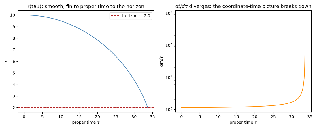
dt/dtau near the start of the fall: 1.1180
dt/dtau near the horizon:            185.6897  (still climbing -- diverges exactly at r=2M)

The true singularity: reached analytically, not numerically

The closed-form proper time to r=0 follows from the same radial energy-conservation equation the integrator solves, independent of which time coordinate is used to parametrize the fall – it is larger than the proper time to the horizon found above, exactly as it must be (the particle keeps falling, and keeps accumulating proper time, after crossing the horizon).

tau_r0 = (np.pi / 2.0) * np.sqrt(R0**3 / (2.0 * M))
print(f"\nclosed-form proper time to the TRUE singularity r=0: tau_r=0 = {tau_r0:.4f}")
print(f"proper time to the horizon found numerically above:            tau_horizon = {tau[-1]:.4f}")
print(f"tau_horizon < tau_r=0: {tau[-1] < tau_r0}  (the particle keeps falling, and keeps aging, past the horizon)")
print("\nPenrose's actual theorem needs none of this machinery -- no radial symmetry, no explicit")
print("solution, and no coordinate system at all: once a trapped surface forms, SOME causal geodesic")
print("must be incomplete, full stop. The finite-tau/divergent-t contrast above is the elementary,")
print("coordinate-bound precursor puzzle that made a fully coordinate-free proof necessary in the first place.")

plt.show()

closed-form proper time to the TRUE singularity r=0: tau_r=0 = 35.1241
proper time to the horizon found numerically above:            tau_horizon = 33.6990
tau_horizon < tau_r=0: True  (the particle keeps falling, and keeps aging, past the horizon)

Penrose's actual theorem needs none of this machinery -- no radial symmetry, no explicit
solution, and no coordinate system at all: once a trapped surface forms, SOME causal geodesic
must be incomplete, full stop. The finite-tau/divergent-t contrast above is the elementary,
coordinate-bound precursor puzzle that made a fully coordinate-free proof necessary in the first place.