Perihelion precession: the anomaly that first confirmed General Relativity

Mercury’s orbit precesses by about 43 arcseconds per century more than Newtonian gravity (including the perturbations of the other planets) can account for – a puzzle known since Le Verrier’s 1859 analysis. Einstein’s 1915 calculation of exactly this excess, from General Relativity alone with no free parameters, was his first observational triumph and a major reason the theory was taken seriously. Unlike a Newtonian ellipse, a bound Schwarzschild orbit of semi-major axis \(a\) and eccentricity \(e\) advances its periapsis by, at leading post-Newtonian order,

\[\Delta\phi = \frac{6\pi M}{a (1 - e^2)}\]

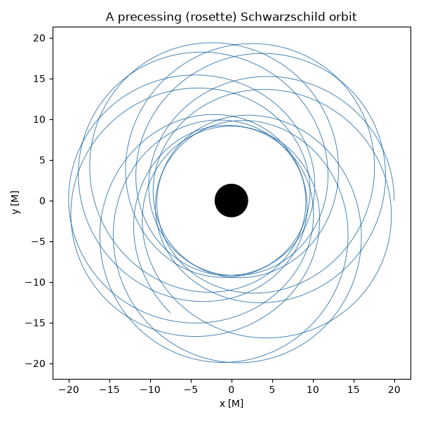
each orbit. This example integrates an eccentric Schwarzschild geodesic exactly (no approximation – solving the full timelike geodesic equation of motion) and measures its perihelion precession directly from the trajectory, comparing against this leading-order post-Newtonian formula. To make the (otherwise tiny) effect visible, the orbit used here is deliberately far more relativistic than Mercury’s, starting much closer to the black hole.

import matplotlib.pyplot as plt
import numpy as np

from physicskit.relativity.chapters.schwarzschild import SchwarzschildBlackHole

Integrate an eccentric orbit and watch it precess

bh = SchwarzschildBlackHole(M=1.0)
y0 = bh.eccentric_orbit_initial_state(r0=20.0, eccentricity_boost=0.15)
traj = bh.integrate_geodesic(y0, dtau=0.02, n_steps=200000)

fig, ax = plt.subplots(figsize=(6, 6))
x = traj["r"] * np.cos(traj["phi"])
y = traj["r"] * np.sin(traj["phi"])
ax.plot(x, y, linewidth=0.7, color="steelblue")
circle = plt.Circle((0, 0), bh.horizon_radius, color="black")
ax.add_patch(circle)
ax.set_aspect("equal")
ax.set_xlabel("x [M]")
ax.set_ylabel("y [M]")
ax.set_title("A precessing (rosette) Schwarzschild orbit")
plt.tight_layout()

Measure the precession per orbit and compare to the weak-field formula

precession = bh.perihelion_precession(traj)
if len(precession) == 0:
    print("No full periapsis passage completed -- increase n_steps to see precession.")
else:
    e_est = (traj["r"].max() - traj["r"].min()) / (traj["r"].max() + traj["r"].min())
    a_semi = (traj["r"].max() + traj["r"].min()) / 2.0
    weak_field = bh.weak_field_precession_per_orbit(a_semi, e_est)
    print(f"Measured precession per orbit: {np.degrees(np.mean(precession)):.3f} deg")
    print(f"Leading-order PN estimate:     {np.degrees(weak_field):.3f} deg")
    print("(Mercury's actual GR excess is only ~43 arcsec/century -- this orbit is")
    print(" deliberately much closer to a strong-field black hole to make the effect visible.)")

Measured precession per orbit: 139.731 deg
Leading-order PN estimate:     86.128 deg
(Mercury's actual GR excess is only ~43 arcsec/century -- this orbit is
 deliberately much closer to a strong-field black hole to make the effect visible.)

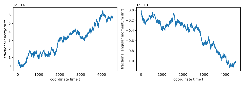
Energy and angular momentum conservation (integration accuracy check)

fig, axes = plt.subplots(1, 2, figsize=(10, 3.5))
axes[0].plot(traj["t"], (traj["energy"] - traj["energy"][0]) / traj["energy"][0])
axes[0].set_xlabel("coordinate time t")
axes[0].set_ylabel("fractional energy drift")
axes[1].plot(
    traj["t"],
    (traj["angular_momentum"] - traj["angular_momentum"][0]) / traj["angular_momentum"][0],
)
axes[1].set_xlabel("coordinate time t")
axes[1].set_ylabel("fractional angular momentum drift")
plt.tight_layout()
plt.show()