The ADM (3+1) formalism: black-hole initial data and the ADM mass

Arnowitt, Deser and Misner (1959-1962) split spacetime into a stack of spatial slices. Each slice carries a 3-metric \(\gamma_{ij}\) and extrinsic curvature \(K_{ij}\), and a lapse \(\alpha\) and shift \(\beta^i\) say how the next slice is laid on top:

\[ds^2 = -\alpha^2dt^2 + \gamma_{ij}(dx^i+\beta^idt)(dx^j+\beta^jdt).\]

Einstein’s equations become evolution equations plus four constraints every slice must satisfy. ADM also defined the total mass of an isolated spacetime from the falloff of \(\gamma_{ij}\) far away. This example builds the simplest nontrivial slices: a moment of time symmetry (\(K_{ij}=0\)) with a conformally flat metric \(\gamma_{ij}=\psi^4\delta_{ij}\), for which the Hamiltonian constraint reduces to \(\nabla^2\psi = 0\). It checks that Schwarzschild in isotropic coordinates, \(\psi=1+M/2r\), satisfies it, then builds Brill-Lindquist two-black-hole data and measures its ADM mass numerically.

import matplotlib.pyplot as plt
import numpy as np

One black hole: Schwarzschild on a slice

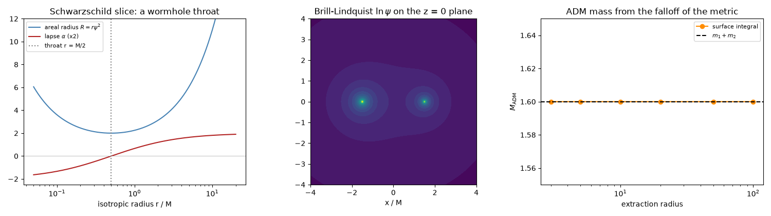
With \(\psi = 1 + M/2r\), the areal radius is \(R = r\psi^2 = r(1+M/2r)^2\), which has a minimum of \(2M\) at \(r = M/2\): the slice is an Einstein-Rosen bridge between two asymptotically flat ends, with the horizon at the throat. The static lapse \(\alpha = (1-M/2r)/(1+M/2r)\) reproduces the Schwarzschild \(g_{tt}\) and vanishes exactly there.

M = 1.0
r = np.geomspace(0.05, 20, 600)
psi = 1 + M / (2 * r)
R_areal = r * psi**2
alpha = (1 - M / (2 * r)) / (1 + M / (2 * r))
print(f"minimum areal radius {R_areal.min():.4f} at r = {r[np.argmin(R_areal)]:.3f}  (2M = {2 * M}, M/2 = {M / 2})")
print(f"-alpha^2 vs Schwarzschild g_tt = -(1 - 2M/R): max difference {np.max(np.abs(alpha**2 - (1 - 2 * M / R_areal))):.1e}")

minimum areal radius 2.0000 at r = 0.499  (2M = 2.0, M/2 = 0.5)
-alpha^2 vs Schwarzschild g_tt = -(1 - 2M/R): max difference 5.1e-16

Two black holes: Brill-Lindquist data

Because \(\nabla^2\psi = 0\) is linear, superposing punctures gives valid initial data for any number of black holes at rest: \(\psi = 1 + \sum_i m_i/(2|\mathbf r-\mathbf r_i|)\). Check the Hamiltonian constraint with a finite-difference Laplacian on a 3D grid.

masses = [(1.0, np.array([-1.5, 0, 0])), (0.6, np.array([1.5, 0, 0]))]


def psi_BL(X, Y, Z):
    out = np.ones_like(X)
    for m, c in masses:
        out += m / (2 * np.sqrt((X - c[0]) ** 2 + (Y - c[1]) ** 2 + (Z - c[2]) ** 2))
    return out


h = 0.05
g = np.arange(-6, 6 + h / 2, h)
z_slab = h * np.arange(-2, 3) + h / 3  # thin slab through the punctures' plane, offset off the grid points
X, Y, Z = np.meshgrid(g, g, z_slab, indexing="ij")
P = psi_BL(X, Y, Z)
lap = (
    (P[2:, 1:-1, 1:-1] + P[:-2, 1:-1, 1:-1] - 2 * P[1:-1, 1:-1, 1:-1])
    + (P[1:-1, 2:, 1:-1] + P[1:-1, :-2, 1:-1] - 2 * P[1:-1, 1:-1, 1:-1])
    + (P[1:-1, 1:-1, 2:] + P[1:-1, 1:-1, :-2] - 2 * P[1:-1, 1:-1, 1:-1])
) / h**2
far = np.min([np.sqrt((X[1:-1, 1:-1, 1:-1] - c[0]) ** 2 + Y[1:-1, 1:-1, 1:-1] ** 2) for _, c in masses], axis=0) > 1.0
print(f"\nHamiltonian constraint residual |lap psi| away from the punctures: max {np.abs(lap[far]).max():.1e} (O(h^2) truncation)")

Hamiltonian constraint residual |lap psi| away from the punctures: max 4.4e-03 (O(h^2) truncation)

The ADM mass

For conformally flat data, \(M_{\rm ADM} = -\frac{1}{2\pi}\oint_{S_\infty}\partial_r\psi\,dA\). Evaluated on spheres of growing radius it converges to \(m_1+m_2\): the total energy, measured from infinity, of two black holes momentarily at rest (their negative interaction energy is already hidden in the bare masses \(m_i\)).

n_th, n_ph = 180, 360
th, ph = np.meshgrid((np.arange(n_th) + 0.5) * np.pi / n_th, np.arange(n_ph) * 2 * np.pi / n_ph, indexing="ij")
n_hat = np.stack([np.sin(th) * np.cos(ph), np.sin(th) * np.sin(ph), np.cos(th)])
radii = np.array([3, 5, 10, 20, 50, 100.0])
M_adm = []
for Rs in radii:
    dR = 1e-4 * Rs
    outer = psi_BL(*(n_hat * (Rs + dR)))
    inner = psi_BL(*(n_hat * (Rs - dR)))
    dpsi_dr = (outer - inner) / (2 * dR)
    dA = Rs**2 * np.sin(th) * (np.pi / n_th) * (2 * np.pi / n_ph)
    M_adm.append(-np.sum(dpsi_dr * dA) / (2 * np.pi))
for Rs, Ma in zip(radii, M_adm):
    print(f"  extraction radius {Rs:5.0f}: M_ADM = {Ma:.5f}")
print(f"  m1 + m2 = {sum(m for m, _ in masses)}")

fig, (ax1, ax2, ax3) = plt.subplots(1, 3, figsize=(15, 4.2))
ax1.plot(r, R_areal, color="steelblue", label="areal radius $R = r\\psi^2$")
ax1.plot(r, 2 * alpha, color="firebrick", label=r"lapse $\alpha$ (x2)")
ax1.axvline(M / 2, color="0.5", ls=":", label="throat r = M/2")
ax1.axhline(0, color="0.7", lw=0.6)
ax1.set_xscale("log")
ax1.set_ylim(-2.5, 12)
ax1.set_xlabel("isotropic radius r / M")
ax1.set_title("Schwarzschild slice: a wormhole throat")
ax1.legend(fontsize=8)
xy = np.linspace(-4, 4, 400)
XX, YY = np.meshgrid(xy, xy, indexing="ij")
ax2.contourf(XX, YY, np.log(psi_BL(XX, YY, 0.01 + 0 * XX)), levels=30, cmap="viridis")
ax2.set_aspect("equal")
ax2.set_title(r"Brill-Lindquist $\ln\psi$ on the z = 0 plane")
ax2.set_xlabel("x / M")
ax3.semilogx(radii, M_adm, "o-", color="darkorange", label="surface integral")
ax3.axhline(sum(m for m, _ in masses), color="k", ls="--", label="$m_1 + m_2$")
ax3.set_xlabel("extraction radius")
ax3.set_ylabel(r"$M_{\rm ADM}$")
ax3.set_ylim(1.55, 1.65)
ax3.set_title("ADM mass from the falloff of the metric")
ax3.legend(fontsize=8)
fig.tight_layout()

plt.show()

extraction radius     3: M_ADM = 1.60001
extraction radius     5: M_ADM = 1.60002
extraction radius    10: M_ADM = 1.60002
extraction radius    20: M_ADM = 1.60002
extraction radius    50: M_ADM = 1.60002
extraction radius   100: M_ADM = 1.60002
m1 + m2 = 1.6

Check

Isotropic Schwarzschild: the areal radius has a minimum 2M at the throat r = M/2; Brill-Lindquist data satisfy the Hamiltonian constraint to O(h^2), and the ADM mass is m1 + m2 at every extraction radius.

assert abs(R_areal.min() - 2 * M) < 1e-3 and abs(r[np.argmin(R_areal)] - M / 2) < 0.01
assert np.max(np.abs(alpha**2 - (1 - 2 * M / R_areal))) < 1e-12
assert np.abs(lap[far]).max() < 1e-2
np.testing.assert_allclose(M_adm, 1.6, rtol=1e-4)