Validating the curvature engine: Einstein’s vacuum field equations

Einstein’s field equations, \(G_{\mu\nu} = 8\pi T_{\mu\nu}\), reduce to \(G_{\mu\nu} = 0\) in vacuum (no matter or energy present). Schwarzschild and Kerr describe the vacuum spacetime outside a mass, so their Einstein tensors must vanish identically everywhere outside the horizon – despite the metrics themselves being far from flat. This example uses physicskit.relativity’s numerical (finite-difference) curvature engine to verify this directly for both metrics at several radii, and shows how the same engine reveals genuine matter content (a nonzero Einstein tensor) for a charged Reissner-Nordstrom black hole, whose electromagnetic field sources spacetime curvature even in the “vacuum” region outside the horizon.

import matplotlib.pyplot as plt
import numpy as np

from physicskit.relativity.core.tensors import (
    einstein_tensor,
    kerr_metric_bl,
    reissner_nordstrom_metric,
    schwarzschild_metric,
)

Schwarzschild and Kerr: vacuum, so G_munu = 0 everywhere outside the horizon

print("Schwarzschild vacuum check (max |G_munu| at each radius):")
for r in [4.0, 6.0, 10.0, 50.0]:
    coords = np.array([0.0, r, np.pi / 3.0, 0.5])
    G = einstein_tensor(schwarzschild_metric, coords, {"M": 1.0})
    print(f"  r={r:>5.1f}M:  max|G_munu| = {np.max(np.abs(G)):.2e}")

print("\nKerr vacuum check (max |G_munu| at each radius, a=0.8):")
for r in [3.0, 5.0, 10.0, 50.0]:
    coords = np.array([0.0, r, np.pi / 3.0, 0.5])
    G = einstein_tensor(kerr_metric_bl, coords, {"M": 1.0, "a": 0.8})
    print(f"  r={r:>5.1f}M:  max|G_munu| = {np.max(np.abs(G)):.2e}")

Schwarzschild vacuum check (max |G_munu| at each radius):
  r=  4.0M:  max|G_munu| = 2.23e-06
  r=  6.0M:  max|G_munu| = 8.25e-08
  r= 10.0M:  max|G_munu| = 1.56e-05
  r= 50.0M:  max|G_munu| = 5.47e-04

Kerr vacuum check (max |G_munu| at each radius, a=0.8):
  r=  3.0M:  max|G_munu| = 1.34e-06
  r=  5.0M:  max|G_munu| = 5.75e-07
  r= 10.0M:  max|G_munu| = 1.37e-05
  r= 50.0M:  max|G_munu| = 9.33e-04

Reissner-Nordstrom: a charged black hole’s electromagnetic field DOES source curvature, even outside the horizon ——————————————————————————–

print("\nReissner-Nordstrom (Q=0.5M): the electromagnetic stress-energy sources G_munu != 0")
for r in [3.0, 5.0, 10.0]:
    coords = np.array([0.0, r, np.pi / 3.0, 0.5])
    G = einstein_tensor(reissner_nordstrom_metric, coords, {"M": 1.0, "Q": 0.5})
    print(f"  r={r:>5.1f}M:  max|G_munu| = {np.max(np.abs(G)):.4f}  (nonzero: matter/field IS present)")

Reissner-Nordstrom (Q=0.5M): the electromagnetic stress-energy sources G_munu != 0
  r=  3.0M:  max|G_munu| = 0.0278  (nonzero: matter/field IS present)
  r=  5.0M:  max|G_munu| = 0.0100  (nonzero: matter/field IS present)
  r= 10.0M:  max|G_munu| = 0.0025  (nonzero: matter/field IS present)

Mapping the vacuum check over the full (r, theta) plane

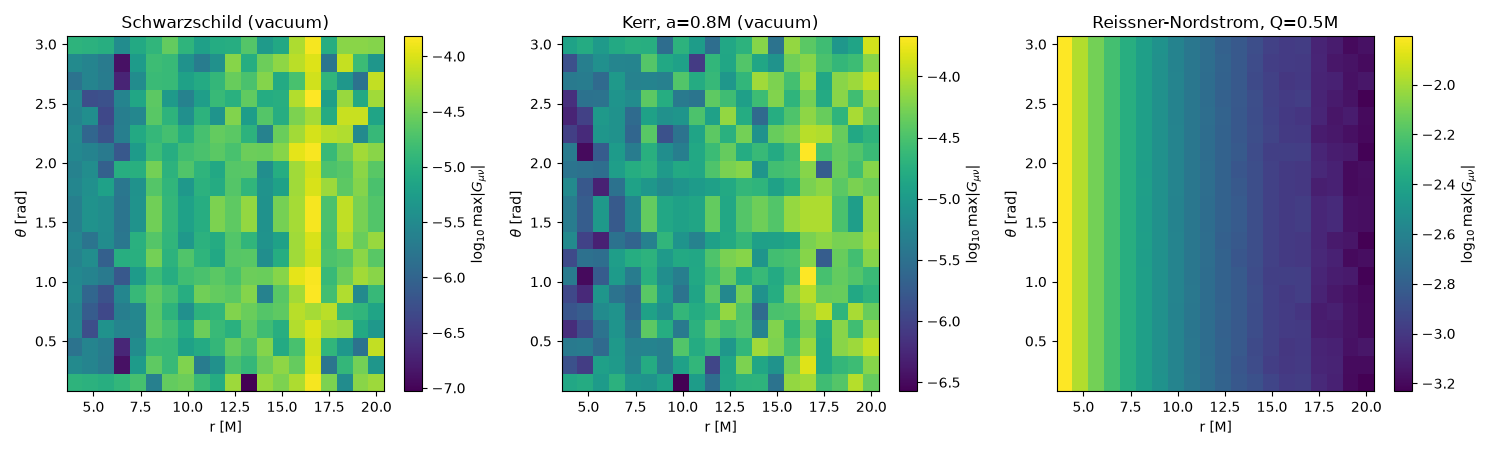
The discrete radii above are single points along one check; evaluating einstein_tensor() over a full grid of \((r,\theta)\) shows the vacuum identity \(G_{\mu\nu}=0\) holds everywhere outside the horizon for both Schwarzschild and Kerr (down to the finite-difference engine’s numerical noise floor), while the Reissner-Nordstrom charge sources a smooth, radius-dependent (and here, theta-independent, since \(Q\) couples only through \(r\)) curvature everywhere – not just at the three sampled radii above.

r_grid = np.linspace(4.0, 20.0, 20)
theta_grid = np.linspace(0.15, np.pi - 0.15, 20)  # stay off the polar coordinate singularity


def _max_G_map(metric_func, params):
    G_map = np.zeros((len(theta_grid), len(r_grid)))
    for i, th in enumerate(theta_grid):
        for j, r in enumerate(r_grid):
            coords = np.array([0.0, r, th, 0.5])
            G_map[i, j] = np.max(np.abs(einstein_tensor(metric_func, coords, params)))
    return G_map


G_schwarzschild = _max_G_map(schwarzschild_metric, {"M": 1.0})
G_kerr = _max_G_map(kerr_metric_bl, {"M": 1.0, "a": 0.8})
G_reissner_nordstrom = _max_G_map(reissner_nordstrom_metric, {"M": 1.0, "Q": 0.5})

fig, axes = plt.subplots(1, 3, figsize=(15, 4.5))
for ax, G_map, title in zip(
    axes,
    [G_schwarzschild, G_kerr, G_reissner_nordstrom],
    ["Schwarzschild (vacuum)", "Kerr, a=0.8M (vacuum)", "Reissner-Nordstrom, Q=0.5M"],
):
    im = ax.pcolormesh(r_grid, theta_grid, np.log10(G_map + 1.0e-300), shading="auto", cmap="viridis")
    plt.colorbar(im, ax=ax, label=r"$\log_{10}\max|G_{\mu\nu}|$")
    ax.set_xlabel("r [M]")
    ax.set_ylabel(r"$\theta$ [rad]")
    ax.set_title(title)
plt.tight_layout()
plt.show()