The Wachter Law for Jacobi Ensembles

The Jacobi (MANOVA) ensemble is built from two independent Wishart-type matrices \(A\) and \(B\), each \(n \times n\) and formed from \(m_1\) and \(m_2\) independent Gaussian “samples” of \(n\) variables respectively (\(m_1, m_2 \geq n\)). The double-Wishart ratio matrix

\[J = A\,(A + B)^{-1}\]

(equivalently, the symmetrized matrix \(M = (A+B)^{-1/2} A (A+B)^{-1/2}\), which is what is actually diagonalized numerically) has real eigenvalues confined to \([0, 1]\) – a “double hard edge” rather than the soft edges of the semicircle or Marchenko-Pastur laws. JOE (\(\beta=1\)) uses real Gaussian entries for \(A, B\); JUE (\(\beta=2\)) uses complex Gaussian entries. The ensembles are indexed by the inverse aspect ratios \(a = m_1/n\) and \(b = m_2/n\) (samples per variable, both \(\geq 1\)).

As \(n \to \infty\) with \(a, b\) fixed, the empirical spectral density converges to the Wachter limiting law. Writing \(s = a+b\), the support edges are

\[\lambda_\pm = \left(\sqrt{\tfrac{a}{s}\left(1-\tfrac{1}{s}\right)} \pm \sqrt{\tfrac{1}{s}\left(1-\tfrac{a}{s}\right)}\right)^2,\]

and the density on \((\lambda_-, \lambda_+)\) is

\[p(x) = \frac{(a+b)\,\sqrt{(x-\lambda_-)(\lambda_+-x)}} {2\pi\, x\,(1-x)}.\]

This example reproduces that law across a few \((a, b)\) pairs.

Reference: K. W. Wachter, Ann. Statist. 8 (1980) 937.

Run:

python examples/paper_replications/wachter_demo.py

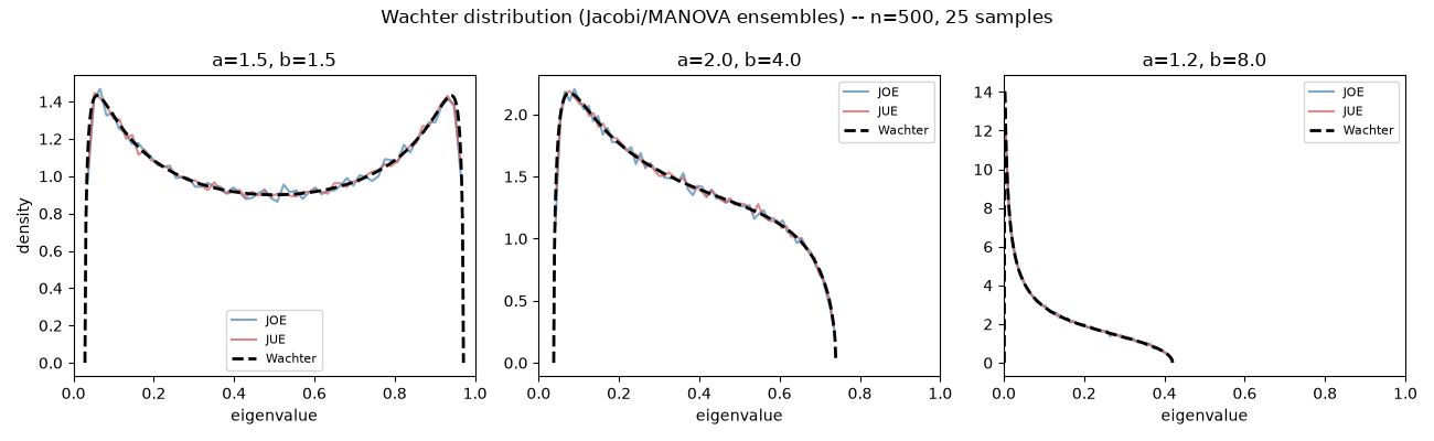
Saved wachter_replication.png

import matplotlib.pyplot as plt
import numpy as np

import physicskit.rmt as rmt

N = 500
N_SAMPLES = 25
SEED = 2026
PAIRS = [(1.5, 1.5), (2.0, 4.0), (1.2, 8.0)]  # (a, b) = (m1/n, m2/n)

fig, axes = plt.subplots(1, len(PAIRS), figsize=(13, 4))

for ax, (a, b) in zip(axes, PAIRS, strict=True):
    m1, m2 = int(a * N), int(b * N)
    benchmark = rmt.validation.Wachter(a=a, b=b)
    lo, hi = rmt.stats.wachter_support(a, b)
    x = np.linspace(lo, hi, 400)

    for cls, color in [(rmt.ensembles.JOE, "steelblue"), (rmt.ensembles.JUE, "indianred")]:
        ensemble = cls(n=N, m1=m1, m2=m2, seed=SEED)
        spectrum = ensemble.sample(n_samples=N_SAMPLES)
        centers, counts = rmt.stats.empirical_density(spectrum, bins=60, rescaled=False)
        ax.plot(centers, counts, color=color, alpha=0.7, lw=1.5, label=cls.__name__)

    ax.plot(x, benchmark.theoretical_pdf(x), "k--", lw=2, label="Wachter")
    ax.set_title(f"a={a}, b={b}")
    ax.set_xlabel("eigenvalue")
    ax.set_xlim(0, 1)
    ax.legend(fontsize=8)

axes[0].set_ylabel("density")
fig.suptitle(f"Wachter distribution (Jacobi/MANOVA ensembles) -- n={N}, {N_SAMPLES} samples")
fig.tight_layout()
out_path = "wachter_replication.png"
fig.savefig(out_path, dpi=150)
print(f"Saved {out_path}")