The Berry-Tabor formula: an integrable billiard’s spectrum

Gutzwiller’s trace formula assumes each periodic orbit is isolated. In an integrable system that fails. Periodic orbits come in continuous families filling whole resonant tori, and the Gutzwiller stability weight \(1/\sqrt{|\det(M-I)|}\) diverges. Berry and Tabor (1976) replaced the sum over isolated orbits with a sum over these families, labelled by integer winding numbers \((M, N)\). Each family adds an oscillation to the density of states with amplitude proportional to the area it sweeps and falling off only as \(L^{-1/2}\) with its length \(L\).

The rectangular billiard (sides \(a, b\)) shows this with exact quantum levels \(k_{mn}^2 = \pi^2(m^2/a^2 + n^2/b^2)\) and periodic-orbit families of length \(L_{MN} = 2\sqrt{(Ma)^2 + (Nb)^2}\). The length spectrum, the Fourier transform of the exact levels in wavenumber, has a peak at each of those lengths. For contrast, this example also evaluates gutzwiller_amplitude_from_monodromy() on a family orbit’s monodromy matrix, which has \(\operatorname{tr}M = 2\), to show where the isolated-orbit formula breaks.

import matplotlib.pyplot as plt
import numpy as np

from physicskit.semiclassical.core.gutzwiller import gutzwiller_amplitude_from_monodromy

a, b = 1.0, (1 + np.sqrt(5)) / 2  # irrational aspect ratio: no accidental degeneracies

Exact levels

m, n = np.meshgrid(np.arange(1, 400), np.arange(1, 400), indexing="ij")
k_all = np.pi * np.sqrt((m / a) ** 2 + (n / b) ** 2)
K_max = 250.0
k = np.sort(k_all[k_all < K_max])
weyl = a * b * k**2 / (4 * np.pi) - 2 * (a + b) * k / (4 * np.pi)
print(f"{k.size} levels below k = {K_max}; Weyl estimate {a * b * K_max**2 / (4 * np.pi) - 2 * (a + b) * K_max / (4 * np.pi):.0f}")

7947 levels below k = 250.0; Weyl estimate 7943

The length spectrum

\(|\sum_n w(k_n)\,e^{ik_nL}|\), with a smooth window \(w\) to suppress ringing from the cutoff. Peaks sit at the family lengths \(L_{MN}\); the Weyl term only contributes near \(L=0\).

L = np.linspace(0.3, 9.0, 3000)
window = np.cos(0.5 * np.pi * k / K_max) ** 2
length_spectrum = np.abs(np.exp(1j * np.outer(L, k)) @ window)
families = {(M, N): 2 * np.hypot(M * a, N * b) for M in range(0, 5) for N in range(0, 4) if (M, N) != (0, 0)}

fig, (ax1, ax2) = plt.subplots(1, 2, figsize=(13, 4.2), gridspec_kw={"width_ratios": [2.2, 1]})
ax1.plot(L, length_spectrum, color="steelblue", lw=1)
for (M, N), LMN in sorted(families.items(), key=lambda kv: kv[1]):
    if LMN < L[-1]:
        ax1.axvline(LMN, color="firebrick", ls=":", lw=0.8)
        ax1.text(LMN, length_spectrum.max() * 1.02, f"({M},{N})", rotation=90, fontsize=7, ha="center", va="bottom")
ax1.set_xlabel("orbit length L")
ax1.set_ylabel("length spectrum")
ax1.set_title("Fourier transform of the exact levels: one peak per orbit family", pad=28)

found = []
for (M, N), LMN in sorted(families.items(), key=lambda kv: kv[1])[:6]:
    window_mask = np.abs(L - LMN) < 0.1
    found.append((M, N, LMN, L[window_mask][np.argmax(length_spectrum[window_mask])]))
print("\nfamily (M,N): predicted length, peak in the length spectrum")
for M, N, LMN, Lpk in found:
    print(f"  ({M},{N}): {LMN:.3f}  {Lpk:.3f}")

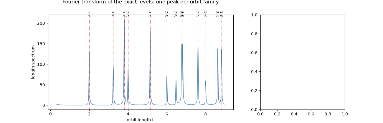
family (M,N): predicted length, peak in the length spectrum
  (1,0): 2.000  2.000
  (0,1): 3.236  3.239
  (1,1): 3.804  3.804
  (2,0): 4.000  4.002
  (2,1): 5.145  5.145
  (3,0): 6.000  6.000

Why Gutzwiller’s weight fails here

A bouncing-ball orbit between the two sides of length \(a\) (family (0,1)) is neutrally stable. Displacing it sideways gives another periodic orbit, so its monodromy matrix is a shear, \(\begin{pmatrix}1&L\\0&1\end{pmatrix}\), with trace 2. The isolated-orbit amplitude \(1/\sqrt{|2-\operatorname{tr}M|}\) is infinite, and a whole family must be summed instead, which is what Berry and Tabor did.

L01 = families[(0, 1)]
for eps in (1e-1, 1e-3, 1e-6):
    M_near = np.array([[1.0 + eps, L01], [0.0, 1.0 / (1.0 + eps)]])  # slightly unstable perturbation
    print(f"trace M = {np.trace(M_near):.8f}: Gutzwiller amplitude {gutzwiller_amplitude_from_monodromy(M_near):.3e}")

trace M = 2.00909091: Gutzwiller amplitude 1.049e+01
trace M = 2.00000100: Gutzwiller amplitude 1.000e+03
trace M = 2.00000000: Gutzwiller amplitude 1.000e+06

Fluctuations about Weyl’s law

The counting function \(N(k)\) minus Weyl’s smooth estimate is the oscillatory part that the Berry-Tabor sum describes. It fluctuates about zero with no trend, and its size grows slowly with \(k\), as the \(L^{-1/2}\) family amplitudes predict.

ax2.plot(k, np.arange(1, k.size + 1) - weyl, color="darkorange", lw=0.6)
ax2.axhline(0, color="k", lw=0.6)
ax2.set_xlabel("wavenumber k")
ax2.set_ylabel("N(k) - Weyl")
ax2.set_title("Spectral fluctuations")
fig.tight_layout()

plt.show()

Check

Weyl’s law with the Dirichlet boundary term counts the levels, and each periodic-orbit family (M, N) of length 2 sqrt((Ma)^2 + (Nb)^2) gives a peak in the length spectrum; the Gutzwiller amplitude 1/sqrt|tr M - 2| diverges for the marginally stable (tr M = 2) orbits of an integrable billiard.

assert abs(k.size - (a * b * K_max**2 / (4 * np.pi) - 2 * (a + b) * K_max / (4 * np.pi))) < 50
for _M, _N, LMN, Lpk in found:
    assert abs(Lpk - LMN) < 0.01
for eps in (1e-1, 1e-3, 1e-6):
    M_near = np.array([[1.0 + eps, L01], [0.0, 1.0 / (1.0 + eps)]])
    assert np.isclose(gutzwiller_amplitude_from_monodromy(M_near), 1 / np.sqrt(abs(np.trace(M_near) - 2)), rtol=1e-6)