Bogomolny’s transfer operator: quantizing a billiard on its boundary

The Gutzwiller trace formula needs every periodic orbit, and for a chaotic system their number grows exponentially with length. Bogomolny (1992) found a way around this. Choose a Poincare surface of section and build the semiclassical propagator from one crossing to the next,

\[T(q,q';E) = \frac{1}{\sqrt{2\pi i\hbar}} \sqrt{\left|\frac{\partial^2 S}{\partial q\,\partial q'}\right|}\, e^{iS(q,q';E)/\hbar - i\pi\nu/2}.\]

Only short orbits, from one crossing to the next, enter \(T\). The levels are the energies where \(T\) has an eigenvalue 1,

\[\det\left[1-T(E)\right]=0,\]

and expanding \(\log\det\) in powers of \(T\) gives back the periodic orbits as products of these short pieces. For a convex billiard the boundary is the section, \(S=\hbar k\ell\) with \(\ell\) the chord length, and \(T\) becomes a matrix of size set by the number of wavelengths around the boundary.

This example applies bogomolny_transfer_operator() and bogomolny_quantization_function() to the integrable disk, whose exact levels are Bessel zeros, and to the chaotic Bunimovich stadium, compared with finite differences (QuantumBilliard).

import matplotlib.pyplot as plt
import numpy as np
from scipy.special import jn_zeros

from physicskit.chaos.quantum.billiards import QuantumBilliard
from physicskit.chaos.systems.billiards import BunimovichStadium
from physicskit.semiclassical.core.bogomolny import bogomolny_quantization_function, bogomolny_transfer_operator


def local_minima(ks, f, threshold=0.3):
    i = np.nonzero((f[1:-1] < f[:-2]) & (f[1:-1] < f[2:]) & (f[1:-1] < threshold))[0] + 1
    return ks[i]

The disk

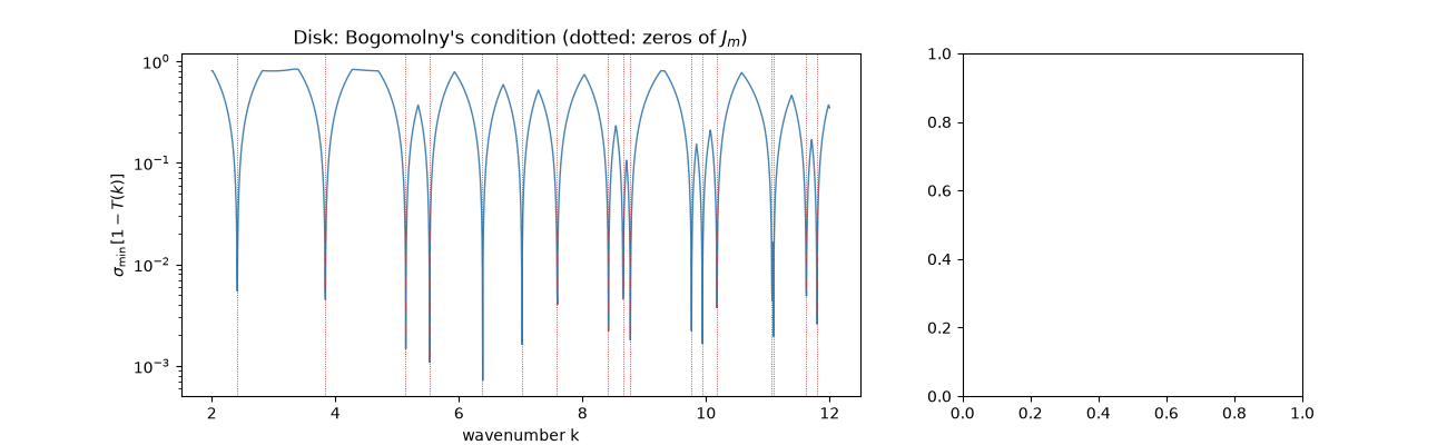
Discretize the unit circle with 120 points (about ten per wavelength at \(k=12\)). The smallest singular value of \(1-T(k)\) dips to nearly zero at each level. The two-fold degenerate levels (\(\pm m\)) show as one dip.

N = 120
phi = 2 * np.pi * np.arange(N) / N
circle = np.column_stack([np.cos(phi), np.sin(phi)])
ds = np.full(N, 2 * np.pi / N)

ks = np.linspace(2.0, 12.0, 2001)
f_disk = bogomolny_quantization_function(ks, circle, -circle, ds)
found = local_minima(ks, f_disk)
exact = np.unique(np.concatenate([jn_zeros(m, 5) for m in range(12)]))
exact = exact[(exact > ks[0]) & (exact < ks[-1])]

fig1, (ax1, ax2) = plt.subplots(1, 2, figsize=(13, 4), gridspec_kw={"width_ratios": [2, 1]})
ax1.semilogy(ks, f_disk, color="steelblue", lw=1)
for k in exact:
    ax1.axvline(k, color="firebrick", lw=0.6, ls=":")
ax1.set_xlabel("wavenumber k")
ax1.set_ylabel(r"$\sigma_{\min}[1-T(k)]$")
ax1.set_title("Disk: Bogomolny's condition (dotted: zeros of $J_m$)")

Text(0.5, 1.0, "Disk: Bogomolny's condition (dotted: zeros of $J_m$)")

At a level an eigenvalue of \(T\) reaches 1. The eigenvalues lie on or inside the unit circle: about \(kL/\pi\) of them, one per propagating direction along the boundary, sit on it, and the rest (evanescent, sub-wavelength structure) collapse to zero.

k_level = jn_zeros(3, 2)[-1]
for k, color, label in [(k_level, "firebrick", f"k = {k_level:.3f} (a level)"), (k_level + 0.25, "0.5", f"k = {k_level + 0.25:.3f}")]:
    ev = np.linalg.eigvals(bogomolny_transfer_operator(circle, -circle, ds, k))
    ax2.plot(ev.real, ev.imag, "o", ms=4, color=color, label=label, zorder=3)
t = np.linspace(0, 2 * np.pi, 300)
ax2.plot(np.cos(t), np.sin(t), "k", lw=0.6)
ax2.plot(1, 0, "o", ms=14, mfc="none", mec="k", zorder=2)
ax2.annotate("eigenvalue 1", (1, 0), (0.3, 0.45), fontsize=8, arrowprops=dict(arrowstyle="->", lw=0.8))
ax2.set_aspect("equal")
ax2.set_title("Eigenvalues of T(k)")
ax2.legend(fontsize=8, loc="lower left")
fig1.tight_layout()

matched = np.array([found[np.argmin(np.abs(found - k))] for k in exact])
print(f"disk: {len(found)} minima for {len(exact)} distinct levels in [2, 12]; max |k_T - k_exact| = {np.max(np.abs(matched - exact)):.4f}")

disk: 17 minima for 17 distinct levels in [2, 12]; max |k_T - k_exact| = 0.0102

The chaotic stadium

Nothing in \(T\) relies on integrability: the chords of the stadium are as easy to write down as those of the disk, although its periodic orbits are unstable and proliferate. The levels of \(\det[1-T]=0\) match the finite-difference spectrum one for one, apart from pairs closer together than the \(k\) grid resolves, with the small upward shift expected at these low \(k\), where the semiclassical approximation is weakest.

R, a = 1.0, 1.0  # cap radius and half the straight length


def stadium_boundary(spacing):
    """Midpoint samples, inward normals and arc-length weights, counterclockwise."""
    n_flat, n_arc = int(np.ceil(2 * a / spacing)), int(np.ceil(np.pi * R / spacing))
    u_flat = (np.arange(n_flat) + 0.5) / n_flat
    u_arc = (np.arange(n_arc) + 0.5) / n_arc
    pieces = []
    for side in (1, -1):  # side = 1: bottom flat then right cap; side = -1: top flat then left cap
        flat = np.column_stack([side * (2 * a * u_flat - a), -side * R * np.ones(n_flat)])
        pieces.append((flat, np.tile([0.0, side], (n_flat, 1)), np.full(n_flat, 2 * a / n_flat)))
        ang = np.pi * u_arc - np.pi / 2 + (0.0 if side == 1 else np.pi)
        cap = np.column_stack([side * a + R * np.cos(ang), R * np.sin(ang)])
        pieces.append((cap, -(cap - [side * a, 0.0]) / R, np.full(n_arc, np.pi * R / n_arc)))
    return (np.vstack([q for q, _, _ in pieces]), np.vstack([n for _, n, _ in pieces]), np.concatenate([w for _, _, w in pieces]))


pts, nrm, ds_st = stadium_boundary(0.05)
ks_st = np.linspace(4.0, 8.0, 801)
f_st = bogomolny_quantization_function(ks_st, pts, nrm, ds_st)
found_st = local_minima(ks_st, f_st)

qb = QuantumBilliard(BunimovichStadium(radius=R, straight_length=2 * a), resolution=300)
eigenvalues, _ = qb.eigenstates(n_states=40)
h = qb.grid()[0][1, 0] - qb.grid()[0][0, 0]
k_fd = 2 / h * np.arcsin(np.sqrt(eigenvalues) * h / 2)  # undo the grid's dispersion
k_fd = k_fd[(k_fd > ks_st[0]) & (k_fd < ks_st[-1])]

fig2, (ax3, ax4) = plt.subplots(1, 2, figsize=(13, 4), gridspec_kw={"width_ratios": [2, 1]})
ax3.semilogy(ks_st, f_st, color="steelblue", lw=1)
for k in k_fd:
    ax3.axvline(k, color="firebrick", lw=0.6, ls=":")
ax3.set_xlabel("wavenumber k")
ax3.set_ylabel(r"$\sigma_{\min}[1-T(k)]$")
ax3.set_title("Stadium: Bogomolny's condition (dotted: finite differences)")
ax4.plot(*np.vstack([pts, pts[:1]]).T, "k", lw=1)
ax4.plot(*pts[::4].T, ".", color="steelblue", ms=3)
for i, j in [(10, 110), (45, 160), (70, 190), (95, 20)]:
    ax4.plot(*pts[[i, j]].T, color="darkorange", lw=0.8)
ax4.set_aspect("equal")
ax4.axis("off")
ax4.set_title(f"Section: {len(pts)} boundary points; a few chords")
fig2.tight_layout()

print(f"stadium: {len(found_st)} minima, {len(k_fd)} finite-difference levels in [4, 8]")
matched_st = np.array([k_fd[np.argmin(np.abs(k_fd - k))] for k in found_st])
print(f"mean shift k_T - k_FD = {np.mean(found_st - matched_st):+.4f}, max |shift| = {np.max(np.abs(found_st - matched_st)):.4f}")

plt.show()

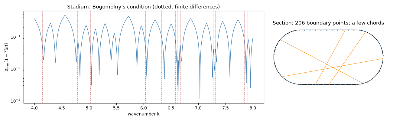
stadium: 22 minima, 24 finite-difference levels in [4, 8]
mean shift k_T - k_FD = +0.0176, max |shift| = 0.0544

Check

det(1 - T(k)) = 0 finds every disk level (zeros of J_m) and, within the boundary discretization error, the stadium levels.

assert len(found) == len(exact) and np.max(np.abs(matched - exact)) < 0.02
assert len(found_st) >= len(k_fd) - 3 and np.max(np.abs(found_st - matched_st)) < 0.06