Gutzwiller’s trace formula: a spectrum from classical orbits

Gutzwiller (1971) wrote the quantum density of states as a smooth part plus one oscillating term for every classical periodic orbit and each of its repetitions. The frequency of each term is set by the orbit’s action, and its weight by the orbit’s period and stability. So the classical orbits encode the quantum spectrum, and the quantum spectrum encodes the orbits.

For the harmonic oscillator every orbit has the same period, which hides most of this. This example uses the pure quartic oscillator \(V=x^4\), whose period shrinks as the energy grows, \(T\propto E^{-1/4}\). Both directions are checked: gutzwiller_density_of_states() builds the spectrum from the orbit, compared with exact levels from NumerovSolver; and a wave packet built from the exact levels revives at multiples of the classical period from classical_period(). Units: \(\hbar = m = 1\).

import matplotlib.pyplot as plt
import numpy as np
from scipy.signal import find_peaks

from physicskit.quantum.core.eigensolvers import NumerovSolver
from physicskit.semiclassical.core.gutzwiller import classical_period, gutzwiller_density_of_states

V = lambda x: x**4  # noqa: E731

Exact spectrum

x = np.linspace(-5, 5, 1601)
exact = NumerovSolver(x, V).solve(n_states=40).energies

The spectrum from one classical orbit and its repetitions

At each energy the trace formula needs only the orbit’s action \(S(E)\) and period \(T(E)\). Summing more repetitions \(r\) sharpens the smooth Weyl density into peaks at the levels.

E_grid = np.linspace(0.2, 14.0, 500)
fig1, ax1 = plt.subplots(figsize=(9, 3.8))
for r_max, color in [(1, "0.6"), (40, "firebrick")]:
    dos = gutzwiller_density_of_states(E_grid, V, 1.0, -5, 5, r_max=r_max, broadening=0.03)
    ax1.plot(E_grid, dos, color=color, lw=1, label=f"repetitions r <= {r_max}")
peaks, _ = find_peaks(dos, height=0.3 * dos.max())
for E in exact[exact < E_grid[-1]]:
    ax1.axvline(E, color="k", lw=0.6, ls=":")
ax1.set_xlabel("energy E")
ax1.set_ylabel("density of states g(E)")
ax1.set_title(r"Quartic oscillator: trace formula (colours) vs exact levels (dotted)")
ax1.legend(fontsize=8)
fig1.tight_layout()

E_sc = E_grid[peaks][: len(exact[exact < E_grid[-1]])]
print(f"{'n':>2s} {'exact':>9s} {'trace formula':>14s} {'rel. diff':>10s}")
for k, (Ee, Es) in enumerate(zip(exact, E_sc)):
    print(f"{k:2d} {Ee:9.4f} {Es:14.4f} {abs(Es / Ee - 1):10.1e}")

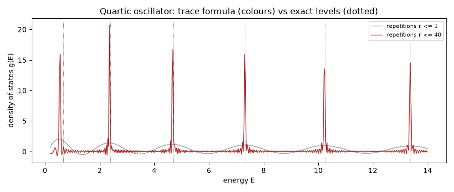
n     exact  trace formula  rel. diff
0    0.6680         0.5595    1.6e-01
1    2.3936         2.3571    1.5e-02
2    4.6968         4.6802    3.5e-03
3    7.3357         7.3074    3.9e-03
4   10.2443        10.2389    5.3e-04
5   13.3793        13.3639    1.2e-03

The orbits from the spectrum: revivals

Superpose exact eigenstates with Gaussian weights centred on level \(n_0\) and follow the autocorrelation \(|\sum_n |c_n|^2 e^{-iE_nt}|^2\). It returns to near 1 each time the classical orbit at that energy closes, at multiples of \(T(E_{n_0})\), the same periods the trace formula summed over. At higher energy the period is shorter.

t = np.linspace(0, 12, 4000)
fig2, ax2 = plt.subplots(figsize=(9, 3.8))
for n0, color in [(10, "steelblue"), (30, "firebrick")]:
    w = np.exp(-0.5 * ((np.arange(len(exact)) - n0) / 2.0) ** 2)
    w /= w.sum()
    C = np.abs(np.exp(-1j * np.outer(t, exact)) @ w) ** 2
    T = classical_period(exact[n0], V, 1.0, -5, 5)
    ax2.plot(t, C, color=color, lw=1, label=f"packet around n = {n0} (E = {exact[n0]:.1f})")
    for r in range(1, int(t[-1] / T) + 1):
        ax2.axvline(r * T, color=color, ls=":", lw=0.8)
    first = t[(t > 0.5 * T) & (t < 1.5 * T)][np.argmax(C[(t > 0.5 * T) & (t < 1.5 * T)])]
    print(f"n0 = {n0}: classical period T(E) = {T:.3f}, first quantum revival at t = {first:.3f}")
ax2.set_xlabel("time t")
ax2.set_ylabel("autocorrelation")
ax2.set_title("Revivals at the classical period (dotted: multiples of T(E))")
ax2.legend(fontsize=8)
fig2.tight_layout()

plt.show()

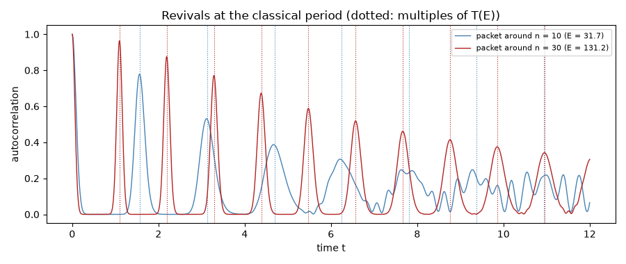
n0 = 10: classical period T(E) = 1.563, first quantum revival at t = 1.560
n0 = 30: classical period T(E) = 1.096, first quantum revival at t = 1.095

Check

The periodic-orbit sum reproduces the quartic levels, better as n grows, and wave packets revive at the classical period T(E).

rel = np.abs(E_sc / exact[: len(E_sc)] - 1)
assert np.all(rel[2:] < 5e-3) and rel[1] < 0.02
for n0 in (10, 30):
    w = np.exp(-0.5 * ((np.arange(len(exact)) - n0) / 2.0) ** 2)
    C = np.abs(np.exp(-1j * np.outer(t, exact)) @ (w / w.sum())) ** 2
    T = classical_period(exact[n0], V, 1.0, -5, 5)
    window = (t > 0.5 * T) & (t < 1.5 * T)
    assert abs(t[window][np.argmax(C[window])] / T - 1) < 0.01