Gutzwiller’s trace formula

Reconstructs the quantum density of states \(g(E)=\sum_n\delta(E-E_n)\) of a unit-mass, unit-frequency harmonic oscillator, \(V(x)=\tfrac12m\omega^2x^2\) with \(m=\omega=\hbar=1\), purely from its classical period \(T(E)\) and action \(S(E)\), with no reference to the quantum eigenstates themselves (classical_period(), gutzwiller_density_of_states()). A bound 1D system has exactly one periodic orbit per energy, so Poisson-summing the discrete Bohr-Sommerfeld spectrum over its repetitions \(r\) gives an identity that is exact here – not merely leading order in \(\hbar\):

\[g(E) = \frac{T(E)/2}{\pi\hbar}\left[1 + 2\sum_{r=1}^{\infty} \cos\!\left(\frac{2rS(E)}{\hbar} - r\pi\right)\right].\]

Truncating the sum at a finite number of repetitions turns each delta function into a finite peak, and those peaks land squarely on the exact Bohr-Sommerfeld energies \(E_n=\hbar\omega(n+\tfrac12)\). Also shows how, for the isolated unstable periodic orbits of a general (chaotic, higher-dimensional) system, the Gutzwiller amplitude

\[\frac{1}{\sqrt{|2-\operatorname{tr}M|}}\]

falls off as the orbit’s monodromy matrix \(M\) becomes more unstable (gutzwiller_amplitude_from_monodromy()).

import matplotlib.pyplot as plt
import numpy as np
from scipy.signal import find_peaks

from physicskit.quantum.chapters.harmonic_spin import HarmonicOscillator
from physicskit.semiclassical.core.gutzwiller import (
    classical_period,
    gutzwiller_amplitude_from_monodromy,
    gutzwiller_density_of_states,
)

ho = HarmonicOscillator()


def V(x):
    return 0.5 * ho.m * ho.omega**2 * x**2


x_min, x_max = -20.0, 20.0

E_values = np.linspace(0.3, 3.0, 60)
periods = [classical_period(E, V, ho.m, x_min, x_max, ho.hbar) for E in E_values]

E_grid = np.linspace(0.2, 6.5, 1200)
dos = gutzwiller_density_of_states(E_grid, V, ho.m, x_min, x_max, hbar=ho.hbar)
peak_idx, _ = find_peaks(dos, height=0.3 * dos.max())
peak_E = E_grid[peak_idx]
bohr_sommerfeld = ho.energy(np.arange(6))

traces = np.linspace(-3, 1.9, 200)
amplitudes = [
    gutzwiller_amplitude_from_monodromy(np.array([[np.exp(0.5 * (2 - tr)), 0.0], [0.0, np.exp(-0.5 * (2 - tr))]])) if tr < 2 else np.nan for tr in traces
]

The (energy-independent) classical period, the reconstructed density of states with peaks landing on the exact spectrum, and the Gutzwiller stability amplitude for an isolated unstable orbit ————————————————————————–

fig, axes = plt.subplots(1, 3, figsize=(15, 4.5))

axes[0].plot(E_values, periods)
axes[0].axhline(2 * np.pi / ho.omega, color="gray", ls="--", label=r"exact $T=2\pi/\omega$")
axes[0].set_xlabel("E")
axes[0].set_ylabel("T(E)")
axes[0].set_title("Classical period (harmonic oscillator:\nindependent of E)")
axes[0].legend(fontsize=8)

axes[1].plot(E_grid, dos, lw=1)
for E_n in bohr_sommerfeld:
    axes[1].axvline(E_n, color="gray", ls=":", lw=0.8)
axes[1].plot(peak_E, dos[peak_idx], "o", color="red", label="reconstructed peaks")
axes[1].set_xlabel("E")
axes[1].set_ylabel("g(E)")
axes[1].set_title("Gutzwiller trace formula: exact 1D\ndensity of states")
axes[1].legend(fontsize=8)

axes[2].plot(traces, amplitudes)
axes[2].set_xlabel(r"tr M")
axes[2].set_ylabel(r"$1/\sqrt{|2-\mathrm{tr}\,M|}$")
axes[2].set_title("Stability amplitude falls off\nfor more unstable orbits")

fig.tight_layout()

print("Reconstructed peaks:      ", np.round(peak_E, 3))
print("Bohr-Sommerfeld spectrum: ", np.round(bohr_sommerfeld, 3))

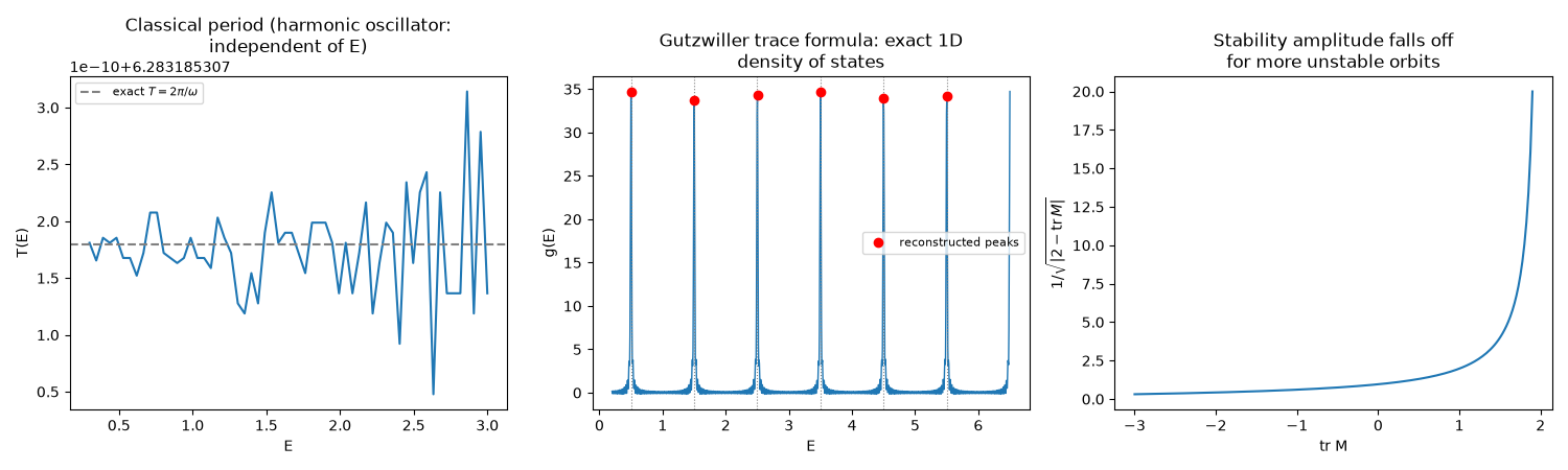
Reconstructed peaks:       [0.499 1.498 2.501 3.5   4.498 5.502]
Bohr-Sommerfeld spectrum:  [0.5 1.5 2.5 3.5 4.5 5.5]