The Van Vleck-Morette propagator beyond quadratic potentials

Van Vleck (1928) showed that, to leading order in \(\hbar\), the quantum propagator is built from classical trajectories alone:

\[K(x,t;x_0,0) \approx \sqrt{\frac{1}{2\pi i\hbar\,|\partial x/\partial p_0|}}\; e^{iS(x,t;x_0)/\hbar - i\mu\pi/2}.\]

For the free particle and the harmonic oscillator this is exact. For any other potential it is an approximation, and its quality is controlled by \(\hbar\) against the classical action scale. This example uses propagate_trajectory_monodromy_action(), van_vleck_prefactor() and count_caustics() (the pieces van_vleck_propagator_1d() assembles) to build the propagator in a quartic-perturbed well from a fan of trajectories out of every starting point. It integrates a Gaussian wavepacket against it and compares the result with the exact split-operator solution (SplitOperatorSolver1D) for decreasing \(\hbar\).

import matplotlib.pyplot as plt
import numpy as np
from numba import njit

from physicskit.quantum.core.solvers import SplitOperatorSolver1D
from physicskit.semiclassical.core.propagators import count_caustics, propagate_trajectory_monodromy_action, van_vleck_prefactor

lam = 0.15
params = np.array([lam])


@njit
def V(q, params):
    return 0.5 * q**2 + params[0] * q**4


@njit
def dVdx(q, params):
    return q + 4 * params[0] * q**3


@njit
def d2Vdx2(q, params):
    return 1.0 + 12 * params[0] * q**2


m, t_final, steps = 1.0, 0.6, 200
dt = t_final / steps
q_c, p_c, sigma = 1.2, 0.0, 0.25
x = np.linspace(-4, 4, 512)
dx = x[1] - x[0]


def psi0(xx, hbar):
    return (2 * np.pi * sigma**2) ** -0.25 * np.exp(-((xx - q_c) ** 2) / (4 * sigma**2) + 1j * p_c * xx / hbar)


def trajectory_fans():
    """For each start x0, a fan of trajectories: final position, action, dq_t/dp0 and Maslov index."""
    x0_grid = np.linspace(q_c - 4 * sigma, q_c + 4 * sigma, 81)
    p0_fan = np.linspace(-6, 6, 481)
    fans = []
    for x0 in x0_grid:
        rows = []
        for p0 in p0_fan:
            q_t, _, M, S, Mqp_hist = propagate_trajectory_monodromy_action(x0, p0, dVdx, d2Vdx2, V, m, dt, steps, params)
            if count_caustics(Mqp_hist) == 0:  # keep the single-valued branch before any focal point
                rows.append((q_t, S, M[0, 1], 0))
        rows = np.array(sorted(rows))
        fans.append((x0, rows))
    return fans, x0_grid[1] - x0_grid[0]


def semiclassical_packet(hbar, fans, dx0):
    """psi(x, t) = integral K_VV(x, t; x0) psi0(x0) dx0.

    The action S and dq_t/dp0 vary smoothly along each fan, so they are
    interpolated onto the x grid; the rapidly varying phase exp(iS/hbar)
    is formed only afterwards.
    """
    psi = np.zeros_like(x, dtype=complex)
    for x0, rows in fans:
        q_t, S, Mqp, mu = rows.T
        inside = (x > q_t[0]) & (x < q_t[-1])
        S_x = np.interp(x[inside], q_t, S)
        amp = np.array([van_vleck_prefactor(mq, hbar) for mq in np.interp(x[inside], q_t, Mqp)])
        mu_x = np.round(np.interp(x[inside], q_t, mu))
        psi[inside] += amp * np.exp(1j * (S_x / hbar - np.pi / 4 - mu_x * np.pi / 2)) * psi0(x0, hbar) * dx0
    return psi


def exact_packet(hbar):
    solver = SplitOperatorSolver1D(x, lambda xx: 0.5 * xx**2 + lam * xx**4, hbar=hbar, m=m, dt=t_final / 2000)
    frames, _ = solver.propagate(psi0(x, hbar), 2000, save_every=2000)
    return frames[-1]

Semiclassical against exact

The packet is followed for \(t = 0.6\), a tenth of a small-amplitude oscillation. The fastest trajectories in a quartic well oscillate faster; any that have already passed a focal point are dropped from the fan, keeping the branch where exactly one trajectory reaches each final point. The fidelity \(|\langle\psi_{\rm exact}|\psi_{\rm VV}\rangle|^2\) approaches 1 as \(\hbar\) shrinks, because the quartic term’s corrections come in at higher order in \(\hbar\).

fans, dx0 = trajectory_fans()
fig, axes = plt.subplots(1, 3, figsize=(14, 3.8), sharey=True)
fidelity = {}
for ax, hbar in zip(axes, (1.0, 0.3, 0.1)):
    psi_sc, psi_ex = semiclassical_packet(hbar, fans, dx0), exact_packet(hbar)
    psi_sc /= np.sqrt(np.sum(np.abs(psi_sc) ** 2) * dx)
    psi_ex /= np.sqrt(np.sum(np.abs(psi_ex) ** 2) * dx)
    fidelity[hbar] = abs(np.sum(psi_ex.conj() * psi_sc) * dx) ** 2
    ax.plot(x, np.abs(psi_ex) ** 2, color="k", lw=3, alpha=0.35, label="exact (split operator)")
    ax.plot(x, np.abs(psi_sc) ** 2, color="firebrick", label="Van Vleck-Morette")
    ax.plot(x, np.abs(psi0(x, hbar)) ** 2, ":", color="0.5", label="t = 0")
    ax.set_title(rf"$\hbar$ = {hbar}: fidelity {fidelity[hbar]:.4f}")
    ax.set_xlabel("x")
    ax.set_xlim(-2.5, 2.5)
axes[0].set_ylabel(rf"$|\psi(x, t={t_final})|^2$")
axes[0].legend(fontsize=8)
fig.suptitle(r"Wavepacket in $V = x^2/2 + 0.15\,x^4$ from classical trajectories")
fig.tight_layout()
for hbar, F in fidelity.items():
    print(f"hbar = {hbar}: 1 - fidelity = {1 - F:.2e}")

plt.show()

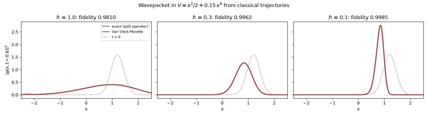
hbar = 1.0: 1 - fidelity = 1.90e-02
hbar = 0.3: 1 - fidelity = 3.81e-03
hbar = 0.1: 1 - fidelity = 1.51e-03

Check

In an anharmonic well the Van Vleck-Morette packet converges to the exact one as hbar -> 0.

infidelity = [1 - fidelity[h] for h in (1.0, 0.3, 0.1)]
assert np.all(np.diff(infidelity) < 0) and infidelity[-1] < 5e-3