The Van Vleck-Morette semiclassical propagator

Reconstructs the quantum propagator of a unit-mass, unit-frequency harmonic oscillator, \(V(q)=\tfrac12 m\omega^2q^2\) with \(m=\omega=1\), from a single classical trajectory alone – no Schrodinger-equation solve involved.

A trajectory launched from \((q_0,p_0)=(1.0,0.3)\) is integrated together with its monodromy matrix \(M(t)=\partial(q_t,p_t)/\partial(q_0,p_0)\) and classical action \(S(t)\) (propagate_trajectory_monodromy_action()), and assembled into the single-trajectory Van Vleck-Morette propagator

\[K(q_t,t;q_0,0) \approx \sqrt{\frac{1}{2\pi\hbar\,|\partial q_t/\partial p_0|}}\, \exp\!\left[\frac{i}{\hbar}S(t) - i\frac{\pi}{4} - i\mu\frac{\pi}{2}\right]\]

(van_vleck_prefactor(), van_vleck_propagator_1d()), where \(\mu\) is the Maslov index – the number of focal points the trajectory has passed through, counted internally with count_caustics() (see The Maslov index: caustics and Keller’s quantization condition for that index’s own topological-invariant story). This is checked against the exact quantum (Mehler) propagator, an exact match here since the oscillator’s quadratic potential makes the WKB expansion behind \(K\) truncate exactly.

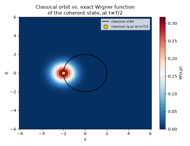
Finally, the same trajectory integrator is re-run from a coherent-state center to trace out a full classical orbit in phase space, which is overlaid directly on the exact quantum Wigner distribution of the coherent state it approximates (plot_classical_trajectory_on_wigner()), showing that the classical orbit is not just a bookkeeping device for the semiclassical amplitude and phase – it traces out exactly where the quantum phase-space distribution’s peak actually sits at each instant.

import matplotlib.pyplot as plt
import numpy as np
from numba import njit

from physicskit.quantum.chapters.harmonic_spin import HarmonicOscillator
from physicskit.semiclassical.core.propagators import (
    propagate_trajectory_monodromy_action,
    van_vleck_propagator_1d,
)
from physicskit.semiclassical.visualizers.propagators import plot_classical_trajectory_on_wigner

m, omega = 1.0, 1.0
params = np.array([m * omega**2])


@njit(cache=True)
def dVdx(q, params):
    return params[0] * q


@njit(cache=True)
def d2Vdx2(q, params):
    return params[0]


@njit(cache=True)
def V(q, params):
    return 0.5 * params[0] * q**2


q0, p0 = 1.0, 0.3
T_period = 2 * np.pi / omega


def exact_propagator(q0, q_t, t):
    return np.sqrt(m * omega / (2j * np.pi * np.sin(omega * t))) * np.exp(
        1j * m * omega / (2 * np.sin(omega * t)) * ((q_t**2 + q0**2) * np.cos(omega * t) - 2 * q_t * q0)
    )


def run(t):
    steps = 4000
    dt = t / steps
    q_t, K = van_vleck_propagator_1d(q0, p0, dVdx, d2Vdx2, V, m, dt, steps, hbar=1.0, params=params)
    return q_t, K


# Before the first caustic (t < T/2, where Mqp=sin(omega*t)/(m*omega) never
# crosses zero) the closed-form Mehler kernel above is single-valued, so it
# is a clean check of the semiclassical propagator; past a caustic, matching
# it would require analytically continuing sqrt(1/sin(omega*t)) across its
# branch cut, which this simple reference formula does not do.
times_compare = np.linspace(0.03, 0.47, 40) * T_period
K_semiclassical, K_exact = [], []
for t in times_compare:
    q_t, K = run(t)
    K_semiclassical.append(K)
    K_exact.append(exact_propagator(q0, q_t, t))
K_semiclassical = np.array(K_semiclassical)
K_exact = np.array(K_exact)

The Van Vleck-Morette propagator’s magnitude and phase against the exact quantum (Mehler) propagator, before the first caustic ————————————————————————–

fig, axes = plt.subplots(1, 2, figsize=(10, 4.5))

axes[0].plot(times_compare / T_period, np.abs(K_exact), label="exact |K|")
axes[0].plot(times_compare / T_period, np.abs(K_semiclassical), "--", label="semiclassical |K|")
axes[0].set_xlabel("t / T")
axes[0].set_title("Propagator magnitude\n(before the first caustic)")
axes[0].legend(fontsize=8)

axes[1].plot(times_compare / T_period, np.angle(K_exact), label="exact phase")
axes[1].plot(times_compare / T_period, np.angle(K_semiclassical), "--", label="semiclassical phase")
axes[1].set_xlabel("t / T")
axes[1].set_title("Propagator phase\n(before the first caustic)")
axes[1].legend(fontsize=8)

fig.tight_layout()

print(f"max |K_semiclassical - K_exact| before the first caustic: {np.max(np.abs(K_semiclassical - K_exact)):.2e}")

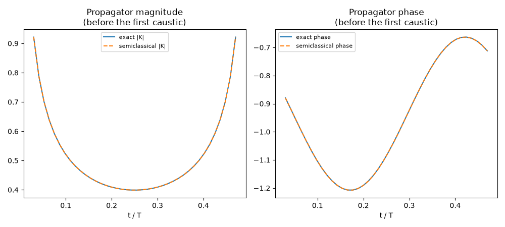
max |K_semiclassical - K_exact| before the first caustic: 1.97e-14

The classical phase-space orbit against the exact quantum Wigner function

Repeatedly re-running the same trajectory integrator used above – propagate_trajectory_monodromy_action() – from a coherent-state center \((q_c,p_c)\) up to increasingly many time steps traces out the full classical orbit over one period, which is then overlaid on the exact Wigner distribution of the coherent state at each point along it.

ho = HarmonicOscillator()
gamma = 1.0 / (2 * ho.x0**2)

qc0, pc0 = 2.0, 0.0
alpha = qc0 / (ho.x0 * np.sqrt(2)) + 1j * pc0 / np.sqrt(2 * ho.hbar * ho.m * ho.omega)
t_half = 0.5 * T_period

n_orbit = 81
t_orbit = np.linspace(0.0, T_period, n_orbit)
dt_orbit = T_period / 2000
q_orbit, p_orbit = [qc0], [pc0]
for t in t_orbit[1:]:
    steps_i = max(1, round(t / dt_orbit))
    q_t, p_t, _, _, _ = propagate_trajectory_monodromy_action(qc0, pc0, dVdx, d2Vdx2, V, m, dt_orbit, steps_i, params)
    q_orbit.append(q_t)
    p_orbit.append(p_t)
q_orbit, p_orbit = np.array(q_orbit), np.array(p_orbit)
idx_half = int(np.argmin(np.abs(t_orbit - t_half)))

x_wigner = np.linspace(-6, 6, 70)
psi_wigner = ho.coherent_wavefunction(alpha, x_wigner, t=t_half)

fig2, ax2 = plt.subplots(figsize=(6.5, 5))
plot_classical_trajectory_on_wigner(x_wigner, psi_wigner, q_orbit, p_orbit, hbar=ho.hbar, ax=ax2)
ax2.plot(q_orbit[idx_half], p_orbit[idx_half], "o", color="gold", mec="k", ms=9, label="classical (q,p) at t=T/2")
ax2.set_ylim(-6, 6)
ax2.set_title("Classical orbit vs. exact Wigner function\nof the coherent state, at t=T/2")
ax2.legend(fontsize=8)
fig2.tight_layout()