Berry’s random-wave conjecture for chaotic eigenfunctions

Berry (1977) conjectured that a high-lying eigenfunction of a classically chaotic system looks locally like a random superposition of plane waves, all with the same wavenumber \(k\) and directions spread uniformly around the circle:

\[\psi(\mathbf r) \approx \sqrt{\frac{2}{NA}}\sum_{j=1}^{N} \cos(k\,\hat{\mathbf n}_j\cdot\mathbf r + \phi_j).\]

The idea is semiclassical. The Wigner function of an eigenstate concentrates where the classical orbits at that energy go, and an ergodic orbit visits every point with every direction of momentum equally. Two predictions follow: the amplitudes \(\psi(\mathbf r)\) are Gaussian distributed, and the spatial autocorrelation is the average of \(\cos(k\hat{\mathbf n}\cdot\Delta\mathbf r)\) over directions, \(J_0(k|\Delta\mathbf r|)\).

This example tests both on eigenstates of the chaotic Bunimovich stadium computed with QuantumBilliard, and contrasts them with an eigenstate of the integrable disk, which is not random. Scars, the exceptions Heller found in 1984, are where the conjecture fails.

import matplotlib.pyplot as plt
import numpy as np
from scipy.special import j0, jn, jn_zeros

from physicskit.chaos.quantum.billiards import QuantumBilliard
from physicskit.chaos.systems.billiards import BunimovichStadium

qb = QuantumBilliard(BunimovichStadium(radius=1.0, straight_length=2.0), resolution=260)
eigenvalues, eigenfunctions = qb.eigenstates(n_states=120)
X, Y = qb.grid()
h = X[1, 0] - X[0, 0]
inside = ~np.isnan(eigenfunctions[0])
# Correct the finite-difference dispersion: the grid Laplacian's eigenvalue
# k_fd^2 corresponds to a slightly larger physical wavenumber.
k_states = 2 / h * np.arcsin(np.sqrt(eigenvalues) * h / 2)

A chaotic eigenstate next to a random wave

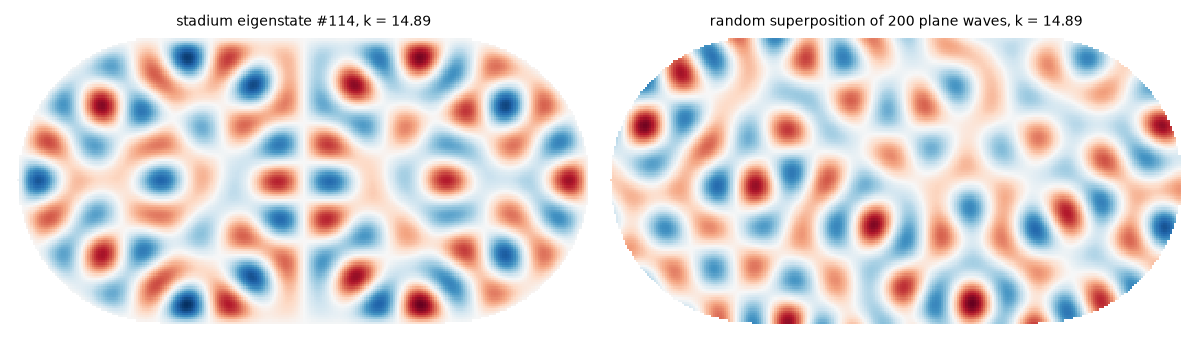
Apart from the mirror symmetries the stadium imposes (every eigenstate is even or odd about both axes), neither picture has any visible order. The random wave is built from 200 plane waves at the eigenstate’s wavenumber, with random directions and phases. Not every stadium state looks like this: state #101, for instance, is a bouncing-ball scar, one of the exceptions to the conjecture.

n_show = 114
k_show = k_states[n_show]
rng = np.random.default_rng(3)
theta = rng.uniform(0, 2 * np.pi, 200)
phases = rng.uniform(0, 2 * np.pi, 200)
random_wave = np.sum(np.cos(k_show * (np.cos(theta)[:, None, None] * X + np.sin(theta)[:, None, None] * Y) + phases[:, None, None]), axis=0)
random_wave[~inside] = np.nan

fig1, axes = plt.subplots(1, 2, figsize=(12, 3.6))
for ax, field, title in [
    (axes[0], eigenfunctions[n_show], f"stadium eigenstate #{n_show}, k = {k_show:.2f}"),
    (axes[1], random_wave, f"random superposition of 200 plane waves, k = {k_show:.2f}"),
]:
    ax.pcolormesh(X, Y, field / np.nanmax(np.abs(field)), cmap="RdBu_r", vmin=-1, vmax=1, shading="auto")
    ax.set_aspect("equal")
    ax.set_title(title, fontsize=10)
    ax.axis("off")
fig1.tight_layout()

Gaussian amplitudes

Pool the normalized amplitudes of 40 stadium eigenstates. Their histogram matches the standard normal density. A disk eigenstate \(J_m(kr)\cos m\phi\) is different: it vanishes inside its caustic circle \(r<m/k\) and its nodal lines form a regular grid of circles and rays, so small amplitudes are far more common than for a Gaussian.

states = range(80, 120)
amplitudes = np.concatenate([eigenfunctions[n][inside] / np.sqrt(np.mean(eigenfunctions[n][inside] ** 2)) for n in states])

m_disk, s_disk = 10, 2
k_disk = jn_zeros(m_disk, s_disk)[-1]
r = np.sqrt(np.random.default_rng(0).uniform(0, 1, 200_000))
phi = np.random.default_rng(1).uniform(0, 2 * np.pi, 200_000)
disk_amp = jn(m_disk, k_disk * r) * np.cos(m_disk * phi)
disk_amp /= np.sqrt(np.mean(disk_amp**2))

u = np.linspace(-4, 4, 400)
fig2, (ax1, ax2) = plt.subplots(1, 2, figsize=(12, 4))
ax1.hist(amplitudes, bins=120, range=(-4, 4), density=True, color="steelblue", alpha=0.6, label="stadium, 40 eigenstates")
ax1.hist(disk_amp, bins=120, range=(-4, 4), density=True, histtype="step", color="darkorange", lw=1.5, label=f"disk, m = {m_disk}, k = {k_disk:.1f}")
ax1.plot(u, np.exp(-(u**2) / 2) / np.sqrt(2 * np.pi), "k", lw=1.5, label="Gaussian (random wave)")
ax1.set_xlabel(r"$\psi/\langle\psi^2\rangle^{1/2}$")
ax1.set_ylabel("probability density")
ax1.set_ylim(0, 0.9)
ax1.set_title("Amplitude distribution")
ax1.legend(fontsize=8)
gauss_small = 0.0797  # P(|z| < 0.1) for a standard normal
print(f"fraction with |psi| < 0.1 rms: stadium {np.mean(np.abs(amplitudes) < 0.1):.3f}, disk {np.mean(np.abs(disk_amp) < 0.1):.3f}, Gaussian {gauss_small}")

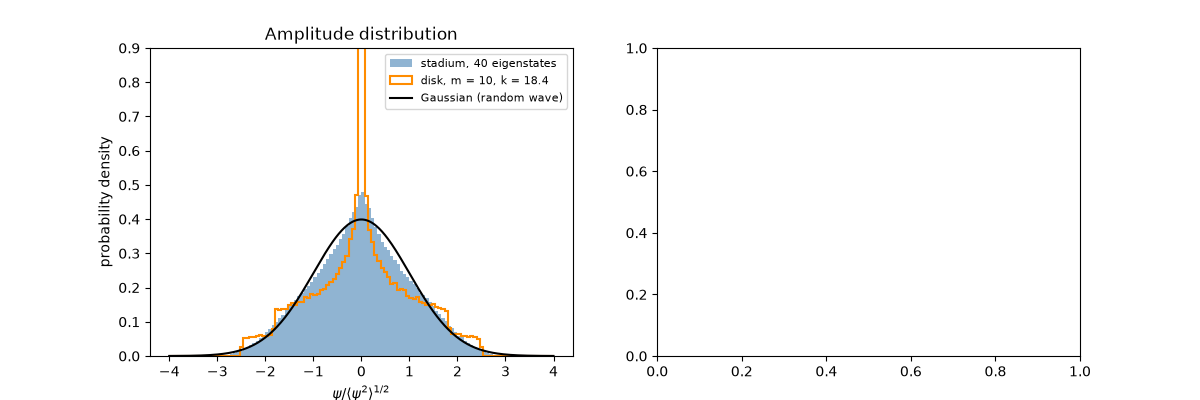
fraction with |psi| < 0.1 rms: stadium 0.093, disk 0.219, Gaussian 0.0797

The autocorrelation is a Bessel function

Correlate each eigenstate with a shifted copy of itself, average over all shift directions, and plot against \(k|\Delta\mathbf r|\). Every stadium state collapses onto Berry’s \(J_0\).

nx, ny = inside.shape
M = inside.astype(float)


def autocorrelation(field):
    F = np.fft.rfft2(field, s=(2 * nx, 2 * ny))
    return np.fft.irfft2(F * np.conj(F), s=(2 * nx, 2 * ny))


overlap = autocorrelation(M)
ix = np.fft.fftfreq(2 * nx) * 2 * nx
iy = np.fft.fftfreq(2 * ny) * 2 * ny
dist = np.hypot(*np.meshgrid(ix, iy, indexing="ij")) * h
usable = overlap > 0.3 * overlap.max()

bins = np.linspace(0, 12, 61)
centres = 0.5 * (bins[1:] + bins[:-1])
for n in range(80, 120, 8):
    field = np.nan_to_num(eigenfunctions[n])
    C = autocorrelation(field) / np.maximum(overlap, 1) / np.mean(eigenfunctions[n][inside] ** 2)
    kr = dist * k_states[n]
    which = np.digitize(kr[usable], bins) - 1
    curve = np.bincount(which, weights=C[usable], minlength=len(bins))[: len(centres)] / np.maximum(np.bincount(which, minlength=len(bins))[: len(centres)], 1)
    ax2.plot(centres, curve, ".", ms=4, label=f"state #{n}")
ax2.plot(centres, j0(centres), "k", lw=1.5, label=r"$J_0(k\,\Delta r)$")
ax2.axhline(0, color="0.7", lw=0.5)
ax2.set_xlabel(r"$k\,|\Delta r|$")
ax2.set_ylabel("direction-averaged autocorrelation")
ax2.set_title("Spatial correlations of stadium eigenstates")
ax2.legend(fontsize=7)
fig2.tight_layout()

plt.show()

Check

Chaotic (stadium) eigenstates look like random waves: Gaussian amplitude statistics and J0(k dr) correlations; the integrable disk’s do not.

assert abs(np.mean(np.abs(amplitudes) < 0.1) - gauss_small) < 0.02
assert np.mean(np.abs(disk_amp) < 0.1) > 2 * gauss_small
assert np.max(np.abs(curve[centres < 8] - j0(centres[centres < 8]))) < 0.1