Heller and Herman-Kluk (1984): spectra from wavepacket recurrences

Heller’s 1984 argument for scars is a statement about wavepackets. Start a Gaussian packet on a periodic orbit of period \(T\). Each time it comes back around, its overlap with its starting state, the autocorrelation \(C(t)=\langle\psi_0|\psi(t)\rangle\), has a recurrence. The Fourier transform of \(C(t)\) is the spectrum weighted by the packet, \(\sum_n|c_n|^2\delta(E-E_n)\). Short-time recurrences at multiples of \(T\) therefore force that weighted spectrum to bunch into bands spaced \(2\pi\hbar/T\), so some eigenstates must carry extra weight on the orbit: a scar. Herman and Kluk’s frozen-Gaussian propagator, published the same year, made such packet dynamics computable semiclassically.

This example applies both ideas to a Morse oscillator, whose exact levels are known. It computes the autocorrelation exactly with SplitOperatorSolver1D and shows how the short-time recurrence sets the smooth spectral envelope while the long-time signal resolves the individual lines. It then propagates the packet over its first quarter-period with herman_kluk_propagate_wavepacket().

import matplotlib.pyplot as plt
import numpy as np
from numba import njit

from physicskit.quantum.core.solvers import SplitOperatorSolver1D
from physicskit.semiclassical.core.propagators import frozen_gaussian_1d, herman_kluk_propagate_wavepacket

D_e, a_m = 8.0, 0.5  # Morse well depth and range; hbar = m = 1
omega0 = a_m * np.sqrt(2 * D_e)
n = np.arange(0, int(np.sqrt(2 * D_e) / a_m - 0.5) + 1)
E_exact = omega0 * (n + 0.5) - (omega0 * (n + 0.5)) ** 2 / (4 * D_e)

x = np.linspace(-6, 30, 2048)
dx = x[1] - x[0]
q0, gamma = 1.5, 1.0
psi0 = frozen_gaussian_1d(x, q0, 0.0, gamma)
dt = 0.005
solver = SplitOperatorSolver1D(x, lambda xx: D_e * (1 - np.exp(-a_m * xx)) ** 2, dt=dt)

The autocorrelation function

The packet starts at rest on the outer side of the well. It returns roughly once per classical period (a little longer than the small-oscillation period, since the well softens with energy), never quite completely, because the levels are unevenly spaced.

n_steps = 16000
frames, times = solver.propagate(psi0, n_steps, save_every=4)
C = np.array([np.sum(psi0.conj() * f) * dx for f in frames])
T_cl = 2 * np.pi / omega0
print(
    f"small-oscillation period 2 pi / omega = {T_cl:.3f}; first recurrence of |C(t)| at t = "
    f"{times[(times > 0.5 * T_cl) & (times < 1.6 * T_cl)][np.argmax(np.abs(C[(times > 0.5 * T_cl) & (times < 1.6 * T_cl)]))]:.3f}"
)

small-oscillation period 2 pi / omega = 3.142; first recurrence of |C(t)| at t = 3.860

Short times give the envelope, long times give the lines

Fourier-transform \(C(t)\) with a Gaussian time window. A window shorter than one period sees only the initial decay and gives one smooth hump. A window of about two periods sees the first recurrences and already splits the spectrum into peaks spaced by about \(2\pi\hbar/T\), Heller’s point. The full record resolves the individual Morse levels \(E_n=\omega(n+\tfrac12)-\omega^2(n+\tfrac12)^2/4D\).

E = np.linspace(0, D_e, 1500)
fig1, (ax1, ax2) = plt.subplots(1, 2, figsize=(12, 4))
ax1.plot(times, np.abs(C), color="steelblue", lw=0.8)
ax1.set_xlim(0, 12 * T_cl)
ax1.set_xlabel("time t")
ax1.set_ylabel(r"$|\langle\psi_0|\psi(t)\rangle|$")
ax1.set_title("Recurrences near each classical period")
dt_s = times[1] - times[0]
for t_win, color, label in [(0.4 * T_cl, "0.5", "window 0.4 T"), (2.0 * T_cl, "darkorange", "window 2 T"), (times[-1] / 3, "firebrick", "full record")]:
    w = np.exp(-0.5 * (times / t_win) ** 2)
    S = np.real(np.exp(1j * np.outer(E, times)) @ (C * w)) * dt_s
    S = 2 * S - C[0].real * dt_s
    ax2.plot(E, S / S.max(), color=color, label=label)
for En in E_exact:
    ax2.axvline(En, color="k", lw=0.5, ls=":")
ax2.set_xlabel("energy E")
ax2.set_ylabel("local spectrum (scaled)")
ax2.set_title("Fourier transform of C(t); dotted: exact Morse levels")
ax2.legend(fontsize=8)
fig1.tight_layout()

S_full = np.real(np.exp(1j * np.outer(E, times)) @ (C * np.exp(-0.5 * (times / (times[-1] / 3)) ** 2)))
peak_E = [E[i] for i in range(1, len(E) - 1) if S_full[i] > S_full[i - 1] and S_full[i] > S_full[i + 1] and S_full[i] > 0.05 * S_full.max()]
print("spectral peaks:", np.round(peak_E[:5], 3), " exact levels:", np.round(E_exact[:5], 3))

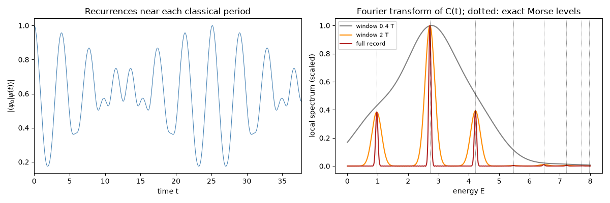
spectral peaks: [0.971 2.716 4.216]  exact levels: [0.969 2.719 4.219 5.469 6.469]

Herman-Kluk over the first quarter-period

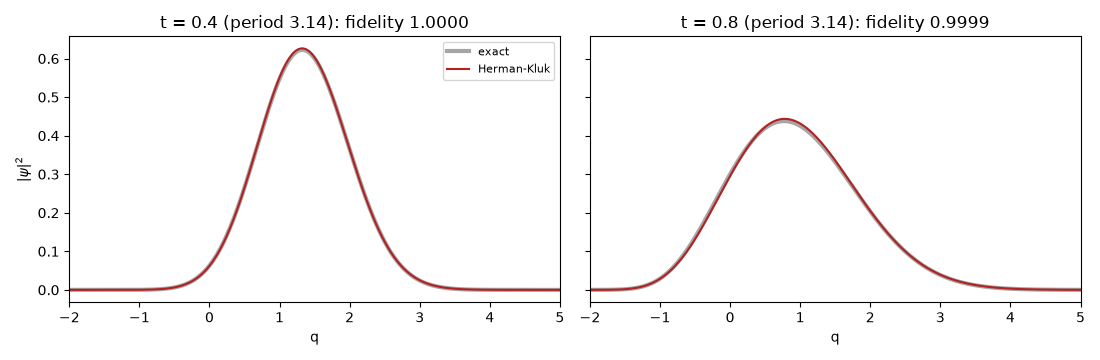
Summing frozen Gaussians launched from a phase-space grid around the initial packet reproduces its early motion and distortion in the anharmonic well. (This finite-grid quadrature of the Herman-Kluk integral is not norm-conserving, and over a full period in this strongly anharmonic well it needs far finer sampling than shown here.)

params = np.array([D_e, a_m])


@njit
def V(q, params):
    return params[0] * (1 - np.exp(-params[1] * q)) ** 2


@njit
def dVdx(q, params):
    e = np.exp(-params[1] * q)
    return 2 * params[0] * params[1] * e * (1 - e)


@njit
def d2Vdx2(q, params):
    e = np.exp(-params[1] * q)
    return 2 * params[0] * params[1] ** 2 * e * (2 * e - 1)


fig2, axes = plt.subplots(1, 2, figsize=(11, 3.6), sharey=True)
for ax, t in zip(axes, (0.4, 0.8)):
    k = int(round(t / dt))
    psi_exact = solver.propagate(psi0, k, save_every=k)[0][-1]
    psi_hk = herman_kluk_propagate_wavepacket(q0, 0.0, gamma, dVdx, d2Vdx2, V, 1.0, dt, k, x, n_grid=41, n_sigma=5.0, params=params)
    fid = abs(np.sum(psi_exact.conj() * psi_hk) * dx) ** 2 / (np.sum(abs(psi_hk) ** 2) * dx)
    print(f"t = {t}: Herman-Kluk fidelity {fid:.4f}")
    ax.plot(x, abs(psi_exact) ** 2, color="k", lw=3, alpha=0.35, label="exact")
    ax.plot(x, abs(psi_hk) ** 2, color="firebrick", label="Herman-Kluk")
    ax.set_xlim(-2, 5)
    ax.set_title(f"t = {t} (period {T_cl:.2f}): fidelity {fid:.4f}")
    ax.set_xlabel("q")
axes[0].set_ylabel(r"$|\psi|^2$")
axes[0].legend(fontsize=8)
fig2.tight_layout()

plt.show()

t = 0.4: Herman-Kluk fidelity 1.0000
t = 0.8: Herman-Kluk fidelity 0.9999

Check

The Fourier transform of C(t) resolves the Morse levels E_n = omega (n + 1/2) - [omega (n + 1/2)]^2 / 4 D_e; |C(t)| recurs at the classical period at the packet’s energy, T(E) = 2 pi / (omega sqrt(1 - E/D_e)), longer than the harmonic 2 pi / omega; Herman-Kluk tracks the packet.

np.testing.assert_allclose(peak_E[:3], E_exact[:3], atol=0.01)
E_packet = 0.5 * gamma + np.sum(np.abs(psi0) ** 2 * D_e * (1 - np.exp(-a_m * x)) ** 2) * dx
window = (times > 0.5 * T_cl) & (times < 1.6 * T_cl)
t_recur = times[window][np.argmax(np.abs(C[window]))]
assert abs(t_recur / (T_cl / np.sqrt(1 - E_packet / D_e)) - 1) < 0.02
assert fid > 0.999