Quantum scars in a chaotic billiard

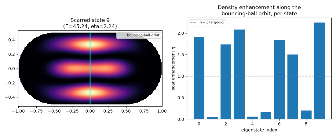
Heller (1984) discovered that individual eigenstates of a classically chaotic system are not always the featureless, ergodically-spread blobs random-matrix intuition suggests: a fraction instead show enhanced probability density concentrated in a tube around one particular unstable classical periodic orbit – a scar.

The system is a Bunimovich stadium billiard (StadiumBilliard2D, \(L=1.0\), \(R=0.5\)): a rectangle of length \(L\) capped by two semicircles of radius \(R\), with an infinite wall at the boundary (\(\psi=0\) outside), whose eigenstates are obtained by direct diagonalization of the 2D finite-difference Laplacian. Its classical dynamics is chaotic, yet one short orbit is only marginally unstable: a trajectory launched perpendicular to the flat top and bottom walls bounces straight up and down forever, blind to \(L\), exactly like a particle in a 1D infinite square well of width \(2R\). Quantizing that motion predicts “bouncing ball” eigenstates near

\[E_n = \frac{(n\pi\hbar)^2}{2m(2R)^2}, \qquad n=1,2,3,\dots,\]

(bouncing_ball_energies()), and the orbit itself is traced with bouncing_ball_orbit_points(). The concentration of density along it is quantified for every computed eigenstate with the enhancement factor

\[\eta = \frac{\langle|\psi|^2\rangle_{\text{tube}}}{\langle|\psi|^2\rangle_{\text{billiard}}},\]

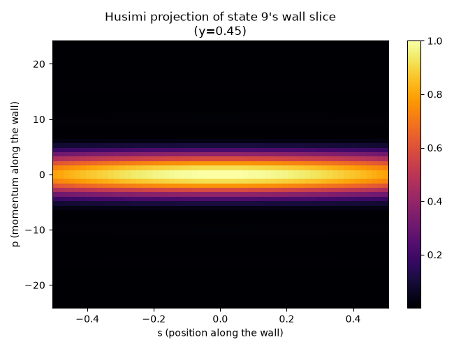
(scar_enhancement()), the ratio of the mean density in a narrow tube around the orbit to the mean density over the whole billiard: \(\eta\approx1\) for an ergodically-spread state and \(\eta\gg1\) for a scarred one. Finally, a 1D slice of the most-scarred state taken along the flat top wall is viewed in phase space with the Husimi (coherent-state) projection husimi_projection_1d(), the same kind of representation Heller used to first see scarring.

import matplotlib.pyplot as plt
import numpy as np

from physicskit.quantum.chapters.potentials import StadiumBilliard2D
from physicskit.semiclassical.systems.scarring import (
    bouncing_ball_energies,
    bouncing_ball_orbit_points,
    husimi_projection_1d,
    scar_enhancement,
)

sb = StadiumBilliard2D(L=1.0, R=0.5)
energies, wavefunctions, Xs, Ys, mask = sb.solve(n_points=220, n_states=10)

predicted = bouncing_ball_energies(sb.R, n_max=4)
print("Predicted bouncing-ball energies:", np.round(predicted, 3))
print("Billiard eigenvalues:            ", np.round(energies, 3))

etas = [scar_enhancement(wf**2, Xs, Ys, mask, x0=0.0, half_width=0.08) for wf in wavefunctions]
scarred_idx = int(np.argmax(etas))
print("Scar enhancement eta per state:", np.round(etas, 2))
print(f"Most scarred state: index {scarred_idx} (E={energies[scarred_idx]:.2f}, eta={etas[scarred_idx]:.2f})")

orbit_x, orbit_y = bouncing_ball_orbit_points(x0=0.0, R=sb.R, n_bounces=3)

Predicted bouncing-ball energies: [ 4.935 19.739 44.413 78.957]
Billiard eigenvalues:             [ 6.249 10.505 17.382 20.947 26.03  26.662 34.121 38.15  44.775 45.238]
Scar enhancement eta per state: [1.91 0.05 1.73 2.08 0.06 0.17 1.84 1.5  0.2  2.24]
Most scarred state: index 9 (E=45.24, eta=2.24)

The most-scarred eigenstate with the bouncing-ball orbit overlaid, and the scar-enhancement factor for every computed eigenstate ————————————————————————–

fig, axes = plt.subplots(1, 2, figsize=(11, 4.5))

density = np.where(mask, wavefunctions[scarred_idx] ** 2, np.nan)
axes[0].pcolormesh(Xs, Ys, density, shading="auto", cmap="magma")
axes[0].plot(orbit_x, orbit_y, color="cyan", lw=1.5, label="bouncing-ball orbit")
axes[0].set_title(f"Scarred state {scarred_idx}\n(E={energies[scarred_idx]:.2f}, eta={etas[scarred_idx]:.2f})")
axes[0].set_aspect("equal")
axes[0].legend(fontsize=8)

axes[1].bar(np.arange(len(etas)), etas)
axes[1].axhline(1.0, color="gray", ls="--", label=r"$\eta=1$ (ergodic)")
axes[1].set_xlabel("eigenstate index")
axes[1].set_ylabel(r"scar enhancement $\eta$")
axes[1].set_title("Density enhancement along the\nbouncing-ball orbit, per state")
axes[1].legend(fontsize=8)

fig.tight_layout()

A Husimi (coherent-state) phase-space projection of a wall slice of the scarred state, near the flat top wall where the bouncing-ball orbit lives ————————————————————————–

x_1d = Xs[:, 0]
y_1d = Ys[0, :]
j_wall = int(np.argmin(np.abs(y_1d - 0.9 * sb.R)))
inside_flat = np.abs(x_1d) <= sb.L / 2
s = x_1d[inside_flat]
psi_wall = wavefunctions[scarred_idx][inside_flat, j_wall].astype(complex)

p_scale = np.sqrt(2 * sb.m * energies[scarred_idx])
S0, P0, husimi = husimi_projection_1d(psi_wall, s, hbar=sb.hbar, p0_range=(-2.5 * p_scale, 2.5 * p_scale))

fig2, ax2 = plt.subplots(figsize=(6.5, 5))
im = ax2.pcolormesh(S0, P0, husimi, shading="auto", cmap="inferno")
ax2.set_xlabel("s (position along the wall)")
ax2.set_ylabel("p (momentum along the wall)")
ax2.set_title(f"Husimi projection of state {scarred_idx}'s wall slice\n(y={y_1d[j_wall]:.2f})")
fig2.colorbar(im, ax=ax2, fraction=0.046)
fig2.tight_layout()