Einstein’s torus quantization: the circular billiard

Sommerfeld quantized each separated coordinate on its own, \(\oint p_i\,dq_i = n_i h\). Einstein (1917) pointed out that this depends on the choice of coordinates, and gave the invariant form: an integrable motion with \(f\) degrees of freedom winds around an \(f\)-dimensional torus in phase space, and the quantization rule is one condition per independent closed loop \(\gamma_i\) on that torus,

\[I_i = \frac{1}{2\pi}\oint_{\gamma_i}\mathbf p\cdot d\mathbf q = \hbar\,(n_i + \alpha_i).\]

The loop integrals do not change when a loop is deformed on the torus, so the rule needs no special coordinates. Einstein also noted that a chaotic orbit, which fills a region instead of a torus, admits no such rule. The offsets \(\alpha_i\) were added by Keller in 1958.

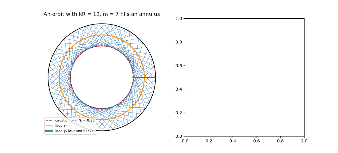
The circular billiard of radius \(R\) shows the torus directly. An orbit with angular momentum \(\hbar m\) never comes closer to the centre than the caustic \(r_c = m/k\), and fills the annulus \(r_c<r<R\). The two loops on its torus give

\[I_\theta = \hbar m,\qquad I_r = \frac{\hbar}{\pi}\left[\sqrt{k^2R^2-m^2} - m\arccos\frac{m}{kR}\right] = \hbar\left(s-\tfrac14\right),\]

with \(\alpha_r = \tfrac14+\tfrac12\) from one caustic and one hard wall. The exact levels are the Bessel zeros \(J_m(kR)=0\).

import matplotlib.pyplot as plt
import numpy as np
from scipy.optimize import brentq
from scipy.special import jn_zeros

R = 1.0


def radial_action(x, m):
    """I_r / hbar as a function of x = k R."""
    return (np.sqrt(x**2 - m**2) - m * np.arccos(m / x)) / np.pi


def torus_levels(m, s_max):
    return np.array([brentq(lambda x: radial_action(x, m) - (s - 0.25), m + 1e-12, m + 4 * s + 10) for s in range(1, s_max + 1)]) / R

An orbit on a torus

A billiard orbit that keeps angular momentum \(m\) bounces between the wall and the caustic circle and, for irrational winding, covers the whole annulus. The two independent loops on the torus are once around the centre (\(\gamma_\theta\)) and once out to the wall and back (\(\gamma_r\)).

k, m = 12.0, 7.0
r_c = m / k
chi = np.arcsin(r_c / R)  # angle between chord and normal
step = np.pi - 2 * chi  # angle advanced per bounce
phi = step * np.arange(60)
bounce = R * np.column_stack([np.cos(phi), np.sin(phi)])

fig1, (ax1, ax2) = plt.subplots(1, 2, figsize=(11, 5))
ax1.plot(*bounce.T, color="steelblue", lw=0.6)
circle = np.linspace(0, 2 * np.pi, 400)
ax1.plot(R * np.cos(circle), R * np.sin(circle), "k", lw=1.5)
ax1.plot(r_c * np.cos(circle), r_c * np.sin(circle), "--", color="firebrick", label=f"caustic r = m/k = {r_c:.2f}")
ax1.plot(0.5 * (R + r_c) * np.cos(circle), 0.5 * (R + r_c) * np.sin(circle), color="darkorange", lw=2, label=r"loop $\gamma_\theta$")
ax1.plot([r_c, R], [0, 0], color="seagreen", lw=3, label=r"loop $\gamma_r$ (out and back)")
ax1.set_aspect("equal")
ax1.set_title(f"An orbit with kR = {k:g}, m = {m:g} fills an annulus")
ax1.legend(fontsize=8, loc="lower left")
ax1.axis("off")

(np.float64(-1.0999674529962649), np.float64(1.0999984501426794), np.float64(-1.0999914757517075), np.float64(1.0999914757517075))

Torus quantization against the exact spectrum

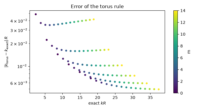
Every level is labelled by its two torus quantum numbers \((m,s)\). The torus rule reproduces the Bessel zeros, and its error falls as \(k\) grows.

m_max, s_max = 14, 6
rows = []
for mm in range(m_max + 1):
    for s, (k_ebk, k_ex) in enumerate(zip(torus_levels(mm, s_max), jn_zeros(mm, s_max)), start=1):
        rows.append((mm, s, k_ebk, k_ex))
rows = np.array(rows)
k_ebk, k_ex = rows[:, 2], rows[:, 3]

ax2.scatter(rows[:, 0], k_ex, s=60, facecolors="none", edgecolors="k", label="exact: zeros of $J_m(kR)$")
ax2.scatter(rows[:, 0], k_ebk, s=12, color="firebrick", label="torus quantization")
ax2.set_xlabel(r"angular quantum number $m$ ($I_\theta=\hbar m$)")
ax2.set_ylabel(r"$kR$")
ax2.set_ylim(0, 25)
ax2.set_title(r"Levels on the $(I_\theta, I_r)$ lattice")
ax2.legend(fontsize=8)
fig1.tight_layout()

fig2, ax3 = plt.subplots(figsize=(7, 3.8))
sc = ax3.scatter(k_ex, np.abs(k_ebk - k_ex), c=rows[:, 0], cmap="viridis", s=14)
ax3.set_yscale("log")
ax3.set_xlabel(r"exact $kR$")
ax3.set_ylabel(r"$|k_{\rm torus}-k_{\rm exact}|\,R$")
ax3.set_title("Error of the torus rule")
fig2.colorbar(sc, ax=ax3, label="m")
fig2.tight_layout()

print(" m  s   torus kR   exact kR")
for mm, s, a, b in rows[(rows[:, 0] <= 2) & (rows[:, 1] <= 3)]:
    print(f"{int(mm):2d} {int(s):2d} {a:10.5f} {b:10.5f}")
low, high = k_ex < 8, k_ex > 16
print(f"mean |error| for kR < 8: {np.mean(np.abs(k_ebk - k_ex)[low]):.4f}; for kR > 16: {np.mean(np.abs(k_ebk - k_ex)[high]):.4f}")

plt.show()

 m  s   torus kR   exact kR
 0  1    2.35619    2.40483
 0  2    5.49779    5.52008
 0  3    8.63938    8.65373
 1  1    3.79444    3.83171
 1  2    6.99700    7.01559
 1  3   10.16093   10.17347
 2  1    5.10039    5.13562
 2  2    8.40014    8.41724
 2  3   11.60825   11.61984
mean |error| for kR < 8: 0.0332; for kR > 16: 0.0099

Check

Einstein-Brillouin-Keller on the disk’s invariant tori reproduces the zeros of J_m, and the error falls as k grows.

assert np.max(np.abs(k_ebk - k_ex)) < 0.06
assert np.mean(np.abs(k_ebk - k_ex)[high]) < 0.5 * np.mean(np.abs(k_ebk - k_ex)[low])