The Langer correction: exact hydrogen levels from radial WKB

The radial equation of a central-force problem looks like a 1D Schrodinger equation on \(r>0\) with the effective potential \(V(r)+\hbar^2 l(l+1)/2mr^2\). Applying the WKB rule \(\int p\,dr=(n_r+\tfrac12)\pi\hbar\) to it gives energies that are wrong even for hydrogen. Langer (1937) traced the problem to the origin: WKB assumes a slowly varying wavelength, which fails near \(r=0\). The substitution \(r=e^x\) maps the half-line onto the full line, where the WKB assumptions hold, and the result is the same as replacing

\[l(l+1)\;\longrightarrow\;\left(l+\tfrac12\right)^2\]

in the centrifugal term. With that one change radial WKB gives the exact hydrogen spectrum \(E=-1/2(n_r+l+1)^2\) (atomic units) and the exact 3D oscillator spectrum \(\hbar\omega(2n_r+l+\tfrac32)\). This example compares both versions using langer_corrected_wkb().

import matplotlib.pyplot as plt
import numpy as np

from physicskit.semiclassical.core.wkb import langer_corrected_wkb

V_coulomb = lambda r: -1.0 / r  # noqa: E731
n_r = np.arange(6)

The two effective potentials

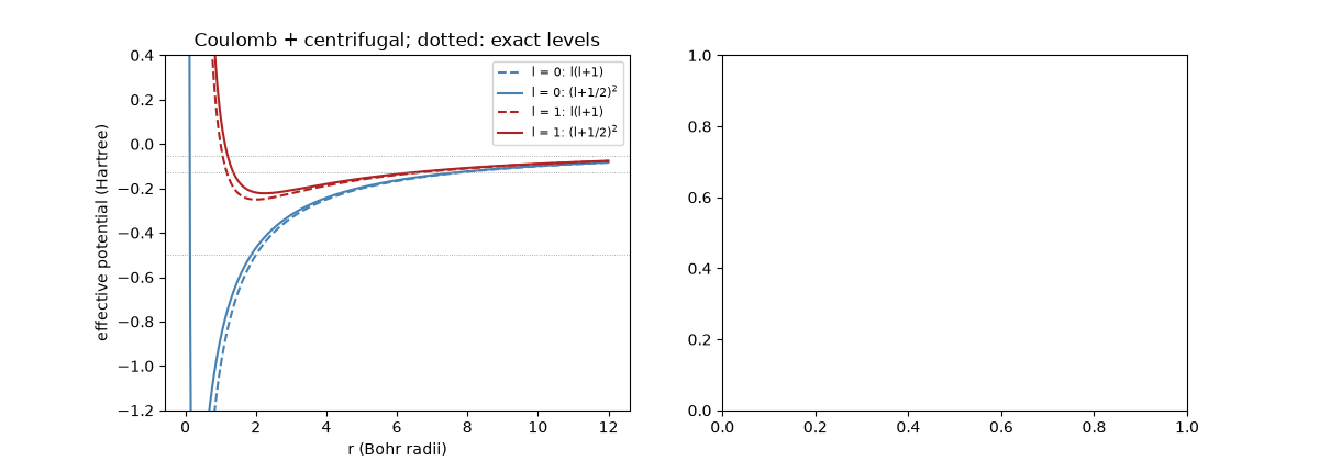
For \(l=0\) the uncorrected potential has no barrier at all, and the WKB integral runs into the Coulomb singularity. Langer’s version always keeps a barrier \(\hbar^2/8mr^2\), which gives a soft inner turning point where the usual connection formula applies.

r = np.linspace(0.02, 12, 600)
fig1, (ax1, ax2) = plt.subplots(1, 2, figsize=(12, 4.2))
for l, color in [(0, "steelblue"), (1, "firebrick")]:
    ax1.plot(r, -1 / r + l * (l + 1) / (2 * r**2), color=color, ls="--", label=f"l = {l}: l(l+1)")
    ax1.plot(r, -1 / r + (l + 0.5) ** 2 / (2 * r**2), color=color, label=f"l = {l}: (l+1/2)$^2$")
for n in range(1, 4):
    ax1.axhline(-0.5 / n**2, color="0.6", lw=0.6, ls=":")
ax1.set_ylim(-1.2, 0.4)
ax1.set_xlabel("r (Bohr radii)")
ax1.set_ylabel("effective potential (Hartree)")
ax1.set_title("Coulomb + centrifugal; dotted: exact levels")
ax1.legend(fontsize=8)

<matplotlib.legend.Legend object at 0x33f9a0f20>

Hydrogen levels with and without the correction

print(" l  n_r   exact        Langer       uncorrected")
for l, color in [(0, "steelblue"), (1, "firebrick"), (2, "seagreen"), (3, "darkorange")]:
    exact = -0.5 / (n_r + l + 1) ** 2
    with_langer = langer_corrected_wkb(V_coulomb, l, m=1.0, r_max=400.0, n_max=len(n_r))
    without = langer_corrected_wkb(V_coulomb, l, m=1.0, r_max=400.0, n_max=len(n_r), langer=False)
    ax2.semilogy(n_r, np.abs(with_langer / exact - 1) + 1e-16, "o-", color=color, label=f"l = {l}, Langer")
    ax2.semilogy(n_r, np.abs(without / exact - 1), "s--", color=color, mfc="none", label=f"l = {l}, l(l+1)")
    for k in range(2):
        print(f"{l:2d} {k:3d} {exact[k]:12.8f} {with_langer[k]:12.8f} {without[k]:12.8f}")
ax2.set_xlabel("radial quantum number $n_r$")
ax2.set_ylabel("relative error of WKB energy")
ax2.set_title("Hydrogen: Langer is exact (to root-finding precision)")
ax2.legend(fontsize=7, ncol=2)
fig1.tight_layout()

l  n_r   exact        Langer       uncorrected
0   0  -0.50000000  -0.50000000  -1.99999999
0   1  -0.12500000  -0.12500000  -0.22222222
1   0  -0.12500000  -0.12500000  -0.13645493
1   1  -0.05555556  -0.05555556  -0.05887450
2   0  -0.05555556  -0.05555556  -0.05747464
2   1  -0.03125000  -0.03125000  -0.03205443
3   0  -0.03125000  -0.03125000  -0.03181855
3   1  -0.02000000  -0.02000000  -0.02029031

The same correction for the 3D harmonic oscillator

Langer’s replacement is not tuned to the Coulomb potential. For \(V=r^2/2\) it also turns radial WKB into the exact spectrum, while the uncorrected version is again off.

V_osc = lambda r: 0.5 * r**2  # noqa: E731
print("\n3D oscillator, l = 2:  exact    Langer    uncorrected")
exact = 2 * n_r[:4] + 2 + 1.5
for e, a, b in zip(exact, langer_corrected_wkb(V_osc, 2, 1.0, 20.0, 4), langer_corrected_wkb(V_osc, 2, 1.0, 20.0, 4, langer=False)):
    print(f"                       {e:6.3f}  {a:8.5f}  {b:8.5f}")

plt.show()

3D oscillator, l = 2:  exact    Langer    uncorrected
                        3.500   3.50000   3.44949
                        5.500   5.50000   5.44949
                        7.500   7.50000   7.44949
                        9.500   9.50000   9.44949

Check

With l(l+1) -> (l+1/2)^2 WKB is exact for hydrogen, -1/2(n_r + l + 1)^2, and for the 3D oscillator, 2 n_r + l + 3/2; without it, it is not.

for l in range(4):
    np.testing.assert_allclose(langer_corrected_wkb(V_coulomb, l, m=1.0, r_max=400.0, n_max=len(n_r)), -0.5 / (n_r + l + 1) ** 2, rtol=1e-6)
    without = langer_corrected_wkb(V_coulomb, l, m=1.0, r_max=400.0, n_max=len(n_r), langer=False)
    assert np.all(np.abs(without / (-0.5 / (n_r + l + 1) ** 2) - 1) > 1e-3)
np.testing.assert_allclose(langer_corrected_wkb(V_osc, 2, 1.0, 20.0, 4), exact, rtol=1e-6)