Weyl’s law: counting levels by phase-space volume

Weyl (1911) proved that the number of eigenvalues of the Laplacian on a membrane of area \(A\) below \(k^2\) grows as

\[N(k) \simeq \frac{A k^2}{4\pi},\]

whatever the membrane’s shape. Read semiclassically, this says each quantum state occupies a phase-space cell of volume \((2\pi\hbar)^d\):

\[N(E) \simeq \frac{\mathrm{Vol}\{(q,p): H(q,p)<E\}}{(2\pi\hbar)^d}.\]

For a billiard (\(E=\hbar^2k^2/2m\)) the volume is the area times a momentum disk of radius \(\hbar k\), giving Weyl’s formula back. For a 1D oscillator the volume is the area enclosed by the orbit, \(\oint p\,dx = 2S(E)\) with \(S\) from wkb_action(). This example checks both. Units: \(\hbar = m = 1\) in 1D, \(\hbar^2/2m = 1\) for the billiards.

import matplotlib.pyplot as plt
import numpy as np
from scipy.special import jn_zeros

from physicskit.quantum.core.eigensolvers import NumerovSolver
from physicskit.semiclassical.core.wkb import turning_points, wkb_action

One dimension: the area inside the orbit

For \(V=x^4\) the levels are not equally spaced, but the count of levels below \(E\) still tracks the phase-space area enclosed by the classical orbit at that energy, divided by \(2\pi\hbar\).

V = lambda x: x**4  # noqa: E731
x = np.linspace(-5, 5, 1601)
levels_1d = NumerovSolver(x, V).solve(n_states=30).energies

E_grid = np.linspace(0.05, levels_1d[-1], 300)
area = np.array([2 * wkb_action(E, V, 1.0, *turning_points(E, V, -5, 5)) for E in E_grid])
weyl_1d = area / (2 * np.pi)

fig1, (ax1, ax2) = plt.subplots(1, 2, figsize=(12, 4))
ax1.step(levels_1d, np.arange(1, len(levels_1d) + 1), where="post", color="k", label="exact staircase N(E)")
ax1.plot(E_grid, weyl_1d, color="firebrick", label=r"$\oint p\,dx\,/\,2\pi\hbar$")
ax1.set_xlabel("energy E")
ax1.set_ylabel("number of levels below E")
ax1.set_title(r"Quartic oscillator $V=x^4$")
ax1.legend(fontsize=8)

# Each level is reached when the enclosed area holds :math:`n+\tfrac12`
# cells (the Bohr-Sommerfeld rule), so the smooth curve passes through the
# middle of every step and the two agree on average.
area_at_levels = np.array([2 * wkb_action(E, V, 1.0, *turning_points(E, V, -5, 5)) for E in levels_1d])
print("cells enclosed at levels n = 0..5:", np.round(area_at_levels[:6] / (2 * np.pi), 3))

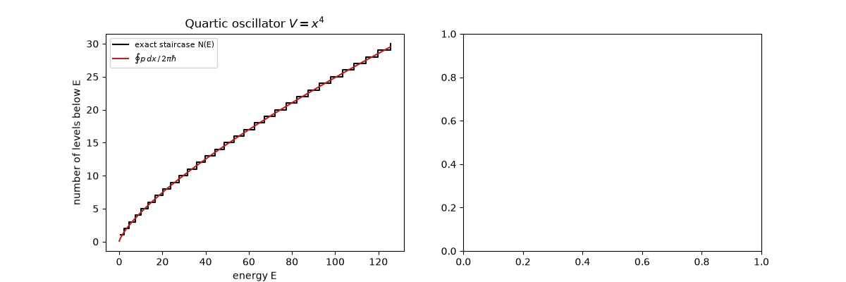
cells enclosed at levels n = 0..5: [0.581 1.514 2.511 3.508 4.506 5.505]

Two dimensions: shape does not matter

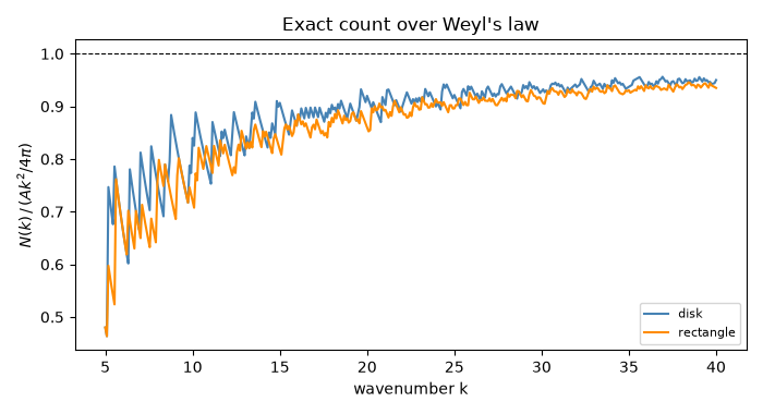
A disk and a rectangle of the same area have completely different spectra (Bessel zeros against sums of squares), yet both counting functions grow with the same \(Ak^2/4\pi\). That shape-independence is Weyl’s theorem.

A = np.pi  # unit disk
k_max = 40.0
disk = []
for m in range(int(k_max) + 1):
    z = jn_zeros(m, int(k_max))
    z = z[z < k_max]
    disk.extend(z if m == 0 else np.repeat(z, 2))
disk = np.sort(disk)

a, b = np.sqrt(A * 2.0), np.sqrt(A / 2.0)  # 2:1 rectangle with area pi
n = np.arange(1, 200)
rect = np.sort((np.pi * np.hypot(n[:, None] / a, n[None, :] / b)).ravel())
rect = rect[rect < k_max]

k = np.linspace(0, k_max, 800)
ax2.step(disk, np.arange(1, len(disk) + 1), where="post", color="steelblue", label=f"unit disk ({len(disk)} levels)")
ax2.step(rect, np.arange(1, len(rect) + 1), where="post", color="darkorange", label=f"2:1 rectangle ({len(rect)} levels)")
ax2.plot(k, A * k**2 / (4 * np.pi), "k--", lw=1, label=r"Weyl $Ak^2/4\pi$")
ax2.set_xlabel("wavenumber k")
ax2.set_ylabel("N(k)")
ax2.set_title(r"Billiards of equal area $A=\pi$")
ax2.legend(fontsize=8)
fig1.tight_layout()

for name, lv in [("disk", disk), ("rectangle", rect)]:
    print(f"{name:9s}: N({k_max:g}) = {len(lv)}, Weyl predicts {A * k_max**2 / (4 * np.pi):.1f}, ratio {len(lv) / (A * k_max**2 / (4 * np.pi)):.3f}")

disk     : N(40) = 380, Weyl predicts 400.0, ratio 0.950
rectangle: N(40) = 374, Weyl predicts 400.0, ratio 0.935

What Weyl’s term leaves out

Divide by the Weyl term and the ratio tends to 1, as the theorem says. The approach is slow, and from below, because the Dirichlet wall removes a strip about half a wavelength wide along the boundary. Balian and Bloch later turned that deficit into the next terms of the expansion.

fig2, ax3 = plt.subplots(figsize=(7, 3.8))
for name, lv, color in [("disk", disk, "steelblue"), ("rectangle", rect, "darkorange")]:
    kk = np.linspace(5, k_max, 400)
    ax3.plot(kk, np.searchsorted(lv, kk) / (A * kk**2 / (4 * np.pi)), color=color, label=name)
ax3.axhline(1, color="k", lw=0.8, ls="--")
ax3.set_xlabel("wavenumber k")
ax3.set_ylabel(r"$N(k)\,/\,(Ak^2/4\pi)$")
ax3.set_title("Exact count over Weyl's law")
ax3.legend(fontsize=8)
fig2.tight_layout()

plt.show()

Check

Each level adds one cell of area 2 pi hbar (n + 1/2 cells at level n, with the Maslov 1/2); billiard counts follow Weyl’s law with the Dirichlet perimeter correction A k^2 / 4 pi - L k / 4 pi.

np.testing.assert_allclose(area_at_levels[1:] / (2 * np.pi), np.arange(1, len(levels_1d)) + 0.5, atol=0.02)
for lv, perimeter in [(disk, 2 * np.pi), (rect, 2 * (a + b))]:
    assert abs(len(lv) - (A * k_max**2 / (4 * np.pi) - perimeter * k_max / (4 * np.pi))) < 5