WKB and Bohr-Sommerfeld quantization

Applies the WKB approximation to a unit-mass, unit-frequency harmonic oscillator, \(V(x)=\tfrac12m\omega^2x^2\) with \(m=\omega=\hbar=1\). Builds the classical momentum

\[p(x) = \sqrt{2m\left(E-V(x)\right)}\]

and its turning points (the roots of \(E=V(x)\)) with classical_momentum() and turning_points(), then builds the WKB standing-wave wavefunction

\[\psi(x) \approx \frac{C}{\sqrt{p(x)}} \cos\!\left(\frac{1}{\hbar}\int_{x_1}^{x}p(x')\,dx' - \frac{\pi}{4}\right)\]

between the two turning points \(x_1,x_2\) (wkb_wavefunction()) and compares it to the exact harmonic-oscillator eigenstate. Finally checks that the Bohr-Sommerfeld (EBK) quantization rule

\[\int_{x_1}^{x_2}p(x)\,dx = \left(n+\tfrac12\right)\pi\hbar, \qquad n=0,1,2,\dots\]

(bohr_sommerfeld_energies()) reproduces the exact spectrum \(E_n=\hbar\omega(n+1/2)\) – the wave- mechanical derivation of the quantization rule that “old quantum theory” had to postulate by hand.

import matplotlib.pyplot as plt
import numpy as np

from physicskit.quantum.chapters.harmonic_spin import HarmonicOscillator
from physicskit.semiclassical.core.wkb import (
    bohr_sommerfeld_energies,
    classical_momentum,
    turning_points,
    wkb_wavefunction,
)

ho = HarmonicOscillator()


def V(x):
    return 0.5 * ho.m * ho.omega**2 * x**2


x_min, x_max = -20.0, 20.0
n_max = 6
energies = bohr_sommerfeld_energies(V, m=ho.m, x_min=x_min, x_max=x_max, n_max=n_max, hbar=ho.hbar)
exact = ho.energy(np.arange(n_max))

The classical momentum and turning points at an example energy, the WKB wavefunction against the exact eigenstate, and the quantized spectrum ————————————————————————–

fig, axes = plt.subplots(1, 3, figsize=(15, 4.5))

E_example = exact[3]
x_p = np.linspace(x_min, x_max, 2000)
p = classical_momentum(E_example, V, x_p, m=ho.m)
tp = turning_points(E_example, V, x_min, x_max)

axes[0].plot(x_p, V(x_p), color="black", lw=1, label="V(x)")
axes[0].axhline(E_example, color="gray", ls="--", label=f"E={E_example:.2f}")
axes[0].plot(x_p, p, label="p(x) (classically allowed region)")
for t in tp:
    axes[0].axvline(t, color="red", ls=":", lw=0.8)
axes[0].set_xlim(-6, 6)
axes[0].set_ylim(-1, 6)
axes[0].set_xlabel("x")
axes[0].set_title("Classical momentum p(x) and turning points")
axes[0].legend(fontsize=8)

n_compare = 5
x_wf = np.linspace(x_min, x_max, 4000)
psi_wkb = wkb_wavefunction(x_wf, exact[n_compare], V, m=ho.m, hbar=ho.hbar)
psi_exact = ho.eigenfunction(n_compare, x_wf)
# Match sign convention for a visual overlay.
if np.dot(psi_wkb, psi_exact) < 0:
    psi_wkb = -psi_wkb
axes[1].plot(x_wf, psi_exact, label=f"exact $\\phi_{n_compare}(x)$", lw=1.5)
axes[1].plot(x_wf, psi_wkb, "--", label=f"WKB $\\psi(x)$, n={n_compare}", lw=1.5)
axes[1].set_xlim(-8, 8)
axes[1].set_xlabel("x")
axes[1].set_title("WKB vs. exact eigenstate")
axes[1].legend(fontsize=8)

axes[2].plot(np.arange(n_max), exact, "o", label=r"exact $\hbar\omega(n+1/2)$")
axes[2].plot(np.arange(n_max), energies, "x", label="Bohr-Sommerfeld (EBK)")
axes[2].set_xlabel("n")
axes[2].set_ylabel("E")
axes[2].set_title("Bohr-Sommerfeld quantization\n(exact for the harmonic oscillator)")
axes[2].legend(fontsize=8)

fig.tight_layout()

print("Bohr-Sommerfeld energies:", np.round(energies, 6))
print("Exact energies:          ", np.round(exact, 6))
print(f"max |EBK - exact|: {np.max(np.abs(energies - exact)):.2e}")

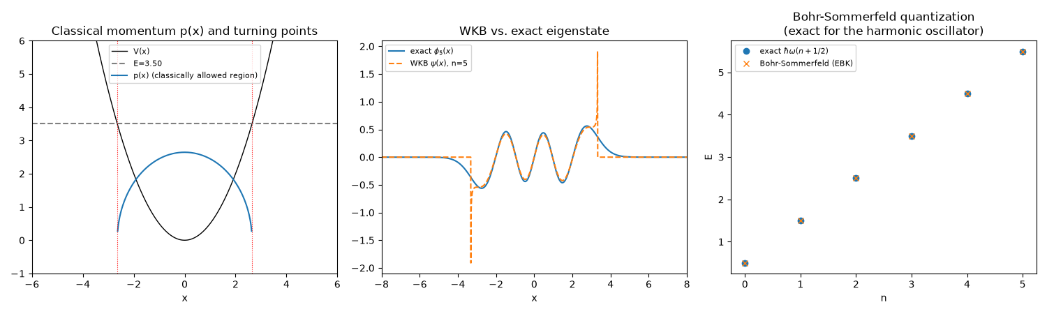
Bohr-Sommerfeld energies: [0.5 1.5 2.5 3.5 4.5 5.5]
Exact energies:           [0.5 1.5 2.5 3.5 4.5 5.5]
max |EBK - exact|: 5.33e-15

Stacking the WKB wavefunction across every quantized level at once

The single-n overlay above only checks one hand-picked level; calling wkb_wavefunction() once per Bohr-Sommerfeld energy and stacking the resulting densities into a single (n, x) image shows that the WKB approximation reproduces the whole ladder of node counts and envelope shapes at once, not just level \(n=5\), together with the per-level WKB-exact overlap this implies.

density_wkb = np.empty((n_max, x_wf.size))
density_exact = np.empty((n_max, x_wf.size))
overlap = np.empty(n_max)
for n in range(n_max):
    psi_n_wkb = wkb_wavefunction(x_wf, exact[n], V, m=ho.m, hbar=ho.hbar)
    psi_n_exact = ho.eigenfunction(n, x_wf)
    if np.dot(psi_n_wkb, psi_n_exact) < 0:
        psi_n_wkb = -psi_n_wkb
    density_wkb[n] = psi_n_wkb**2
    density_exact[n] = psi_n_exact**2
    overlap[n] = np.trapezoid(psi_n_wkb * psi_n_exact, x_wf)

fig2, axes2 = plt.subplots(1, 3, figsize=(15, 4.5))

extent = [x_wf[0], x_wf[-1], -0.5, n_max - 0.5]
# Capped at the (non-divergent) exact density's scale, so the interior node
# structure stays visible; the WKB panel then saturates to bright yellow
# right at the turning points, exactly where wkb_wavefunction's own
# 1/sqrt(p(x)) prefactor is documented to diverge.
vmax = 1.3 * density_exact.max()
axes2[0].imshow(density_wkb, origin="lower", aspect="auto", extent=extent, cmap="viridis", vmax=vmax)
axes2[0].set_xlim(-8, 8)
axes2[0].set_xlabel("x")
axes2[0].set_ylabel("n")
axes2[0].set_title(r"WKB $|\psi_n(x)|^2$, all levels stacked" "\n(saturates at the turning points)")

axes2[1].imshow(density_exact, origin="lower", aspect="auto", extent=extent, cmap="viridis", vmax=vmax)
axes2[1].set_xlim(-8, 8)
axes2[1].set_xlabel("x")
axes2[1].set_ylabel("n")
axes2[1].set_title(r"Exact $|\phi_n(x)|^2$, all levels stacked")

axes2[2].plot(np.arange(n_max), overlap, "o-")
axes2[2].set_ylim(0, 1.05)
axes2[2].set_xlabel("n")
axes2[2].set_ylabel(r"$\langle\psi_{\mathrm{WKB},n}|\phi_n\rangle$")
axes2[2].set_title("WKB-exact overlap, per level")

fig2.tight_layout()

print("WKB-exact overlap per level:", np.round(overlap, 6))

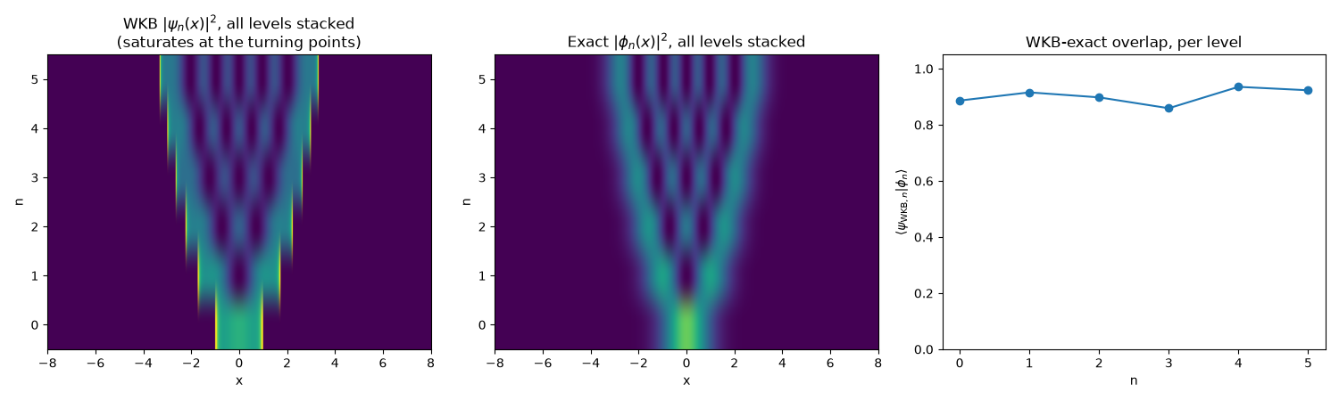
WKB-exact overlap per level: [0.886397 0.915579 0.897817 0.859101 0.935343 0.923097]