Critical slowing down: Metropolis vs. the Wolff cluster algorithm

The 2D Ising model places a spin \(s_i = \pm 1\) on every site of a periodic \(L \times L\) lattice, with Hamiltonian

\[H = -J \sum_{\langle i,j \rangle} s_i s_j,\]

the sum running over nearest-neighbor pairs and \(J > 0\) favoring aligned neighbors. Single-spin-flip Metropolis dynamics decorrelates extremely slowly near a continuous phase transition: the integrated autocorrelation time diverges as \(\tau \sim L^{z}\) with a dynamical critical exponent \(z \approx 2.17\) for 2D Ising Metropolis dynamics. Wolff’s cluster algorithm was invented precisely to defeat this “critical slowing down” by flipping large, physically correlated clusters of aligned spins at once, giving \(z \approx 0.35\) – dramatically faster equilibration at large \(L\). This example measures both algorithms’ integrated autocorrelation times directly at \(T_C\), on an \(L=24\) lattice.

import matplotlib.pyplot as plt
import numpy as np

from physicskit.statphys.chapters.ising_lattice import Ising2D
from physicskit.statphys.utils.dynamics import integrated_autocorrelation_time
from physicskit.statphys.utils.finite_size_scaling import power_law_exponent


def measure_tau(L, algorithm, n_samples, seed=0):
    """Equilibrate an L x L lattice at T_C and measure tau_int of |m| for one algorithm.

    |m| rather than the signed magnetization is used because near T_C the
    *sign* of m performs its own slow random walk under global Z2 symmetry
    (dramatically so under Wolff, whose large cluster flips can reverse the
    sign in a single move); |m| isolates the physically relevant
    order-parameter-magnitude relaxation that critical slowing down affects.
    """
    model = Ising2D(L=L, seed=seed)
    beta = 1.0 / model.T_C
    model.sweep(beta, algorithm=algorithm, n_sweeps=200)  # equilibrate
    series = np.empty(n_samples)
    for k in range(n_samples):
        model.sweep(beta, algorithm=algorithm, n_sweeps=1)
        series[k] = abs(model.magnetization())
    return integrated_autocorrelation_time(series)

Sample magnetization magnitude time series at T_C with each algorithm

L = 24
n_samples = 3000
taus = {}
for algorithm in ["metropolis", "wolff"]:
    taus[algorithm] = measure_tau(L, algorithm, n_samples)
    print(f"{algorithm}: tau_int = {taus[algorithm]:.1f} sweeps (L={L})")

fig, axes = plt.subplots(1, 2, figsize=(9, 4))
axes[0].bar(taus.keys(), taus.values(), color=["steelblue", "crimson"])
axes[0].set_ylabel("integrated autocorrelation time (sweeps)")
axes[0].set_title(f"Critical slowing down at $T_C$, L={L}")
axes[0].set_yscale("log")

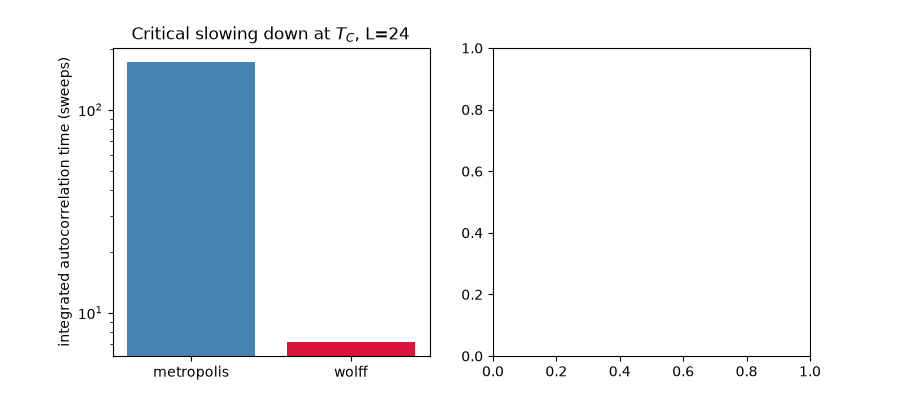
metropolis: tau_int = 171.7 sweeps (L=24)
wolff: tau_int = 7.2 sweeps (L=24)

Dynamical exponent z: how tau_int scales with L

Repeating the same measurement at several smaller lattice sizes (and averaging a handful of independent seeds at each size, since a single tau_int estimate is itself noisy) recovers each algorithm’s dynamical critical exponent from tau_int(L) ~ L^z: Metropolis single-spin-flip dynamics should show z ~ 2.17, dramatically steeper than Wolff cluster flipping’s z ~ 0.35. These modest lattice sizes and sample counts give only a rough estimate of z with visible finite-size bias – exactly the same caveat as the exponent fits in the finite-size-scaling example – but the qualitative gap between the two algorithms is already unmistakable.

L_values = [8, 16, 24]
n_samples_scan = 3000
n_seeds = 4
z_fit = {}
for algorithm, color, marker in zip(["metropolis", "wolff"], ["steelblue", "crimson"], ["o", "s"]):
    tau_L = []
    for L_scan in L_values:
        samples = [measure_tau(L_scan, algorithm, n_samples_scan, seed=s) for s in range(n_seeds)]
        tau_L.append(np.mean(samples))
    z_fit[algorithm], _ = power_law_exponent(L_values, tau_L)
    axes[1].loglog(L_values, tau_L, marker=marker, color=color, label=f"{algorithm} (z={z_fit[algorithm]:.2f})")
    print(f"{algorithm}: fitted dynamical exponent z = {z_fit[algorithm]:.2f} (theory: {2.17 if algorithm == 'metropolis' else 0.35})")

axes[1].set_xlabel("L")
axes[1].set_ylabel(r"$\tau_{\mathrm{int}}(|m|)$ (sweeps)")
axes[1].set_title(r"Dynamical exponent: $\tau_{\mathrm{int}} \sim L^z$")
axes[1].legend(fontsize=8)
plt.tight_layout()
plt.show()

metropolis: fitted dynamical exponent z = 1.59 (theory: 2.17)
wolff: fitted dynamical exponent z = 0.67 (theory: 0.35)